Topics
A monitoring system computes a signature of two thousand features for each machine in a fleet and flags a machine when its nearest neighbours are far away. It is a reasonable design in two dimensions and in ten. In two thousand it flags nothing, or everything, depending on the threshold, because every machine's nearest neighbour is far away, and about as far as its farthest. The failure is not in the data or the code. It is in what distance means when there are many coordinates, and it is worth seeing measured before trusting any method that ranks points by how close they are.
Distances Concentrate
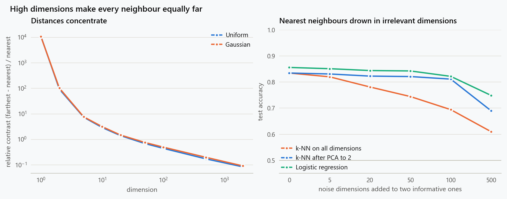
Take $n$ random points and one query point in $d$ dimensions, and compare the distance from the query to its nearest neighbour with the distance to its farthest. The relative contrast is the gap between the two as a share of the nearest distance. Beyer, Goldstein, Ramakrishnan and Shaft showed that under broad conditions it goes to zero as $d$ grows: the farthest point is barely farther than the nearest.
1
2
3
4
5
6
7
8
9
10
11
12
13
14
import numpy as np
from sklearn.neighbors import KNeighborsClassifier, NearestNeighbors
from sklearn.linear_model import LogisticRegression
from sklearn.decomposition import PCA

rng = np.random.default_rng(0)
print("dimension   uniform   gaussian")
for d in (1, 2, 5, 10, 20, 50, 100, 500, 2000):
    out = []
    for gen in (lambda n: rng.uniform(size=(n, d)), lambda n: rng.normal(size=(n, d))):
        X = gen(1000); Q = gen(50)                       # 1,000 points, 50 queries
        D = np.sqrt(((Q[:, None, :] - X[None, :, :]) ** 2).sum(-1))
        out.append(np.mean((D.max(1) - D.min(1)) / D.min(1)))
    print(f"{d:<11}{out[0]:>9.2f}{out[1]:>11.2f}")
| Dimensions | Relative contrast, uniform | Relative contrast, Gaussian |
|---|---|---|
| 1 | 10,867 | 10,578 |
| 2 | 93 | 102 |
| 5 | 7.4 | 7.7 |
| 10 | 2.9 | 3.2 |
| 20 | 1.4 | 1.5 |
| 50 | 0.69 | 0.76 |
| 100 | 0.45 | 0.50 |
| 500 | 0.17 | 0.20 |
| 2,000 | 0.08 | 0.09 |
On a line, a thousand random points leave the nearest neighbour practically on top of the query and the farthest ten thousand times further. In ten dimensions the farthest is three times the nearest. In fifty it is 70 percent farther, and in two thousand it is 8 percent farther. The ranking of a thousand points by distance, which in two dimensions spans two orders of magnitude, has been compressed into a band a few percent wide, and inside that band the order is decided by noise.
The reason is the law of large numbers. A squared Euclidean distance is a sum of $d$ squared coordinate differences. Its mean grows like $d$ and its standard deviation like $\sqrt{d}$, so the spread of distances relative to their size shrinks like $1/\sqrt{d}$. Nothing about the distribution of the points is required beyond the coordinates contributing comparably, and the uniform and Gaussian columns agree because the effect is not about shape.
What It Does to a Nearest-Neighbour Classifier
Two classes separated in two dimensions, with noise dimensions added that carry no information about the class but full weight in the distance.
1
2
3
4
5
6
7
8
9
10
11
12
13
14
15
16
17
18
def dataset(n, noise_dims, r):
    y = r.integers(0, 2, n)
    X = r.normal(size=(n, 2)) + 1.5 * y[:, None] * np.array([1.0, 1.0])
    return np.column_stack([X, r.normal(size=(n, noise_dims))]), y

print("noise dims   kNN   kNN after PCA(2)   logistic")
for nd in (0, 5, 20, 50, 100, 500):
    accs = []
    for rep in range(5):
        r = np.random.default_rng(10 * nd + rep)
        Xtr, ytr = dataset(1000, nd, r); Xte, yte = dataset(2000, nd, r)
        knn = KNeighborsClassifier(5).fit(Xtr, ytr).score(Xte, yte)
        pca = PCA(2, svd_solver="full").fit(Xtr)
        knn_pca = KNeighborsClassifier(5).fit(pca.transform(Xtr), ytr).score(pca.transform(Xte), yte)
        lr = LogisticRegression(max_iter=2000).fit(Xtr, ytr).score(Xte, yte)
        accs.append((knn, knn_pca, lr))
    m = np.mean(accs, axis=0)
    print(f"{nd:<12}{m[0]:.3f}{m[1]:>14.3f}{m[2]:>13.3f}")
| Noise dimensions | k-NN, all dimensions | k-NN after PCA to 2 | Logistic regression |
|---|---|---|---|
| 0 | 0.834 | 0.834 | 0.856 |
| 5 | 0.820 | 0.831 | 0.851 |
| 20 | 0.781 | 0.823 | 0.844 |
| 50 | 0.744 | 0.821 | 0.843 |
| 100 | 0.694 | 0.811 | 0.822 |
| 500 | 0.610 | 0.690 | 0.749 |
The information in the data never changes. With two hundred noise dimensions added, the nearest-neighbour classifier has lost a third of its margin over chance, and with five hundred it is at 61 percent. Its neighbours are chosen by distances in which the two dimensions that matter contribute two parts in five hundred and two, and the neighbours it finds are the points that happen to be close in noise.
Logistic regression degrades far more slowly, because it can learn to put weight near zero on dimensions that do not help; it eventually overfits five hundred coefficients to a thousand examples, which regularisation would repair. Projection to two components holds up through a hundred noise dimensions and then fails, and the reason is instructive: principal components find variance, not relevance. The informative dimensions have slightly more variance than the noise ones, so with few noise dimensions the leading components find them, but with five hundred noise dimensions and a thousand points the sample variance of the noise swamps the difference and the components point nowhere useful. Unsupervised dimensionality reduction cannot tell an informative dimension from a noisy one of the same variance.
What It Does to Anomaly Detection
The monitoring system from the opening scores each machine by its mean distance to its five nearest neighbours. Plant one genuine anomaly, four standard deviations out in the two dimensions that carry the signal, and add irrelevant channels.
1
2
3
4
5
6
7
8
9
10
11
12
print("rank of a planted anomaly's kNN-distance score among 1,000 normal points (1 = most anomalous), 20 repetitions")
for nd in (0, 5, 20, 100, 500):
    ranks = []
    for rep in range(20):
        r = np.random.default_rng(1000 + 100 * nd + rep)
        X = np.column_stack([r.normal(size=(1000, 2)), r.normal(size=(1000, nd))])
        anom = np.concatenate([[4.0, 4.0] / np.sqrt(2), r.normal(size=nd)])
        Xa = np.vstack([X, anom])
        dist, _ = NearestNeighbors(n_neighbors=6).fit(Xa).kneighbors(Xa)
        score = dist[:, 1:].mean(1)
        ranks.append(1 + np.sum(score > score[-1]))
    print(f"  noise dims {nd:>3}: median rank {np.median(ranks):>4.0f} of 1,001, worst {max(ranks):>4}")
| Noise dimensions | Median rank of the anomaly | Worst rank in 20 runs |
|---|---|---|
| 0 | 2 | 3 |
| 5 | 4 | 55 |
| 20 | 62 | 297 |
| 100 | 190 | 644 |
| 500 | 344 | 760 |
With only the two relevant dimensions measured, the planted anomaly is the second most anomalous point of a thousand and one, every time. With twenty irrelevant channels added it is typically the 62nd, and with five hundred it sits in the middle of the pack. Its four-standard-deviation excursion contributes 16 to a squared distance whose typical size is about a thousand, while every normal machine has its own random excursions across five hundred channels that contribute as much. The anomaly is real, is large, and is invisible to the score. Zimek, Schubert and Kriegel's survey of outlier detection in high dimensions is largely a catalogue of this problem and of attempts to route around it.
The Neighbourhood Structure Itself Deforms
Concentration has a second consequence that is easy to miss: the neighbour relation stops being symmetric in a specific, skewed way. Count, for each point, how many other points list it among their ten nearest neighbours.
1
2
3
4
5
6
7
8
9
print("how often the most popular point appears in others' 10 nearest neighbours (1,000 Gaussian points)")
for d in (2, 10, 50, 200, 1000):
    r = np.random.default_rng(d)
    X = r.normal(size=(1000, d))
    _, idx = NearestNeighbors(n_neighbors=11).fit(X).kneighbors(X)
    counts = np.bincount(idx[:, 1:].ravel(), minlength=1000)
    print(f"  d = {d:>4}: max k-occurrence {counts.max():>3} (uniform would be 10), "
          f"share of points never a neighbour {np.mean(counts == 0):.0%}, "
          f"skewness {((counts - counts.mean())**3).mean() / counts.std()**3:.1f}")
| Dimensions | Most popular point appears in this many neighbour lists | Points that appear in none | Skewness of the counts |
|---|---|---|---|
| 2 | 17 | 0% | -0.3 |
| 10 | 41 | 3% | 0.9 |
| 50 | 148 | 13% | 3.7 |
| 200 | 195 | 21% | 4.2 |
| 1,000 | 287 | 30% | 5.3 |
If neighbourhoods were even-handed, each point would appear in about ten lists. In two dimensions the most popular appears in 17 and nobody is left out. In a thousand dimensions one point is a neighbour of 287 others while 30 percent of points are neighbours of no one. Radovanović, Nanopoulos and Ivanović named the popular points hubs and showed they sit near the centre of the data, where concentration makes them slightly closer to everything. Hubs dominate nearest-neighbour votes, so classification errors concentrate around them; clustering methods that rely on density see hubs as cores; and recommendation systems built on item similarity recommend the same few items to everyone. The pathology is a property of the space, and it appears in real high-dimensional data as reliably as in simulated.
What Helps, and What Does Not
Removing irrelevant dimensions helps most. Every table above is a story about dimensions that carry distance but no information. Feature selection with labels, or with domain knowledge about which channels bear on the outcome, attacks the cause. The accuracy table shows the size of the prize: the nearest-neighbour classifier on the two informative dimensions is as good as it ever gets.
Unsupervised projection helps only when the signal has the variance. Principal components find directions of variance, and the table shows them failing once the noise had more. Supervised projections, such as discriminant analysis or a learned metric, find directions of relevance, and they are the right tool when labels exist.
Cosine distance does not escape concentration. It is Euclidean distance between normalised vectors, and normalised vectors concentrate too. It helps when the magnitude of a vector is a nuisance, as with document lengths, and not otherwise. Fractional norms, which Aggarwal, Hinneburg and Keim proposed, retain somewhat more contrast than Euclidean distance; the gain is modest and inconsistent across datasets.
The intrinsic dimension is what counts. Real data with two thousand columns rarely occupies two thousand dimensions. Sensor channels co-vary, image pixels are smooth, and the points lie near a manifold of much lower dimension, and concentration is governed by that dimension rather than by the column count. Estimating it, with methods such as the two-nearest-neighbour estimator of Facco and colleagues, is the first thing to do with a wide table, and it often reveals that a thousand-column dataset behaves like a fifteen-dimensional one, in which distance still works.
Methods that do not rank by distance degrade more gracefully. Trees split on one coordinate at a time and ignore the rest; linear models with regularisation shrink irrelevant coefficients. The logistic column is the mild version of this. They are not immune, as its last row shows, but they fail by overfitting, which is a familiar and treatable failure, rather than by the geometry of the space.
Hubness has its own repairs. Rescaling each distance by the local scale of its endpoints, or replacing distances with shared-nearest-neighbour counts, reduces the skew and improves both classification and clustering in high dimensions.
What to Do
- Count the informative dimensions, not the columns. Estimate the intrinsic dimension before applying any distance-based method.
- Measure the relative contrast on the actual data. If the farthest neighbour is less than twice as far as the nearest, distance rankings are mostly noise.
- Remove or down-weight irrelevant features first, with labels where they exist and with domain knowledge where they do not.
- Do not expect principal components to find relevance. Use a supervised projection when the goal is a distance that respects the outcome.
- Check the k-occurrence distribution for hubs, and apply local scaling or shared-neighbour distances when it is skewed.
- Validate anomaly detectors by planting anomalies of known size and checking their rank, since a detector that cannot find a four-sigma excursion is not going to find a real one.
The nearest-neighbour idea is sound. It just requires that near and far mean something, and past a few dozen dimensions that has to be arranged rather than assumed.
The figure generator in the blog-reproducibility repository reproduces this article's figure; run it with --dry-run to print the numbers behind the figure without writing an image.
References
- Beyer, K., Goldstein, J., Ramakrishnan, R., & Shaft, U. (1999). When is "nearest neighbor" meaningful? In Database Theory, ICDT '99, Lecture Notes in Computer Science 1540, 217-235. Springer.
- Aggarwal, C. C., Hinneburg, A., & Keim, D. A. (2001). On the surprising behavior of distance metrics in high dimensional space. In Database Theory, ICDT 2001, Lecture Notes in Computer Science 1973, 420-434. Springer.
- Radovanović, M., Nanopoulos, A., & Ivanović, M. (2010). Hubs in space: popular nearest neighbors in high-dimensional data. Journal of Machine Learning Research, 11, 2487-2531.
- Zimek, A., Schubert, E., & Kriegel, H.-P. (2012). A survey on unsupervised outlier detection in high-dimensional numerical data. Statistical Analysis and Data Mining, 5(5), 363-387.
- Facco, E., d'Errico, M., Rodriguez, A., & Laio, A. (2017). Estimating the intrinsic dimension of datasets by a minimal neighborhood information. Scientific Reports, 7, 12140.
- Bellman, R. E. (1961). Adaptive Control Processes: A Guided Tour. Princeton University Press.
- Hastie, T., Tibshirani, R., & Friedman, J. (2009). The Elements of Statistical Learning (2nd ed.). Springer.
Embed interactive plots, widgets, and demos using <figure>, <iframe>, or <div class="interactive-embed"> containers. Ensure each embed includes descriptive captions for accessibility.
How to cite
Use the quick export buttons to save citations for reference managers or copy the formatted text directly.
Diogo Ribeiro (2026). Distance Concentration: Why Nearest Neighbours Stop Meaning Anything in High Dimensions. Faculty of Media Arts and Design, Technical University of Porto. https://diogoribeiro7.github.io/mathematics/distance_concentration_high_dimensions/.