Topics
Calculus is built on two operations that turn out to be inverses of each other: differentiation, which measures how fast something changes, and integration, which accumulates change into a total. Almost every quantitative method in data science rests on one or both.
Derivatives: Measuring Change
A derivative measures the rate at which a quantity changes with respect to another variable — how a function's output responds to a change in its input. Geometrically it is the slope of the curve at a point. For a function $f(x)$, the derivative at $x = a$ is the limit
The fraction is the slope of the line through two points on the curve. Taking $h$ to zero slides the second point onto the first, and the secant becomes the tangent. The limit exists only when the curve has a well-defined direction there — which is why $|x|$ has no derivative at zero, and why ReLU networks are technically non-differentiable at the origin, a subtlety handled in practice by picking one of the one-sided slopes.
A positive derivative means the function is increasing; negative means decreasing; zero marks a critical point, which may be a maximum, a minimum, or a saddle. The second derivative distinguishes them: positive means the curve is convex there and the point is a minimum, negative means concave and a maximum. For $f(x) = x^2$ the derivative is $f'(x) = 2x$. At $x = 1$ the slope is 2; at $x = 0$ it is 0, and since $f''(x) = 2 > 0$ everywhere, that critical point is a minimum.
Why Data Science Cares
Nearly all model fitting is minimisation, and minimisation means finding where the derivative vanishes. Gradient descent is the direct application. In several variables the analogue of the derivative is the gradient $\nabla f$, the vector of partial derivatives, which points in the direction of steepest increase. Stepping against it decreases the function:
Backpropagation is the chain rule applied systematically to a composition of functions. If $z = g(h(x))$, then $\frac{dz}{dx} = g'(h(x)) \cdot h'(x)$; a neural network is a long composition, and training it means evaluating that product efficiently from the output backwards. The chain rule also explains vanishing gradients. Multiplying many derivatives each smaller than one drives the product toward zero exponentially in depth, so early layers receive almost no signal — the motivation for ReLU activations, residual connections, and normalisation layers.
1
2
3
4
5
6
7
8
9
10
11
12
13
14
15
import numpy as np

def numerical_gradient(f, x, h=1e-5):
    """Central difference: error is O(h^2), unlike the forward difference."""
    x = np.asarray(x, dtype=float)
    grad = np.zeros_like(x)
    for i in range(x.size):
        step = np.zeros_like(x); step[i] = h
        grad[i] = (f(x + step) - f(x - step)) / (2 * h)
    return grad

f = lambda v: v[0]**2 + 3*v[1]**2 - 2*v[0]*v[1]      # analytic: [2x-2y, 6y-2x]
point = np.array([1.0, 2.0])
print("numerical :", numerical_gradient(f, point).round(6))
print("analytic  :", np.array([2*1 - 2*2, 6*2 - 2*1]))
The central difference is worth knowing beyond textbooks: it is the standard way to verify a hand-derived gradient before trusting it in an optimiser, and a mismatch almost always means an error in the analytic derivation rather than in the approximation.
Choosing $h$ involves a real trade-off. Too large and the approximation is poor; too small and subtracting two nearly equal floating-point numbers loses precision catastrophically. Around $10^{-5}$ balances the two for double precision.
Integrals: Accumulating Quantities
Where the derivative takes a function apart, the integral puts it back together. The definite integral
is the limit of a sum of thin rectangles under the curve — the accumulated total of $f$ across the interval, and geometrically the signed area. The Fundamental Theorem of Calculus ties the two operations together. If $F$ is any antiderivative of $f$, then
which says that accumulating a rate of change over an interval recovers the total change. Differentiation and integration are inverse operations, and that fact is what makes both tractable.
Why Data Science Cares
Probability is where integration earns its place. For a continuous random variable with density $f$,
Every probability statement about a continuous variable is an integral, and the requirement that a density integrates to one is what distinguishes a density from an arbitrary non-negative function. Expectations are integrals too:
This is why Bayesian inference is often computationally demanding. The posterior contains a normalizing constant, the marginal likelihood $\int p(y \mid \theta)p(\theta)\,d\theta$, which is frequently unavailable in closed form. Many Markov Chain Monte Carlo methods avoid evaluating that constant directly: in algorithms such as Metropolis–Hastings, it cancels from the acceptance ratio, allowing samples to be drawn from a posterior known only up to proportionality.
Areas under curves recur in evaluation as well: ROC AUC and PR AUC are exactly what their names say.
1
2
3
4
5
6
7
8
9
10
11
12
from scipy import integrate, stats

# P(-1.96 <= Z <= 1.96) for a standard normal, three ways
exact = stats.norm.cdf(1.96) - stats.norm.cdf(-1.96)
quad, _ = integrate.quad(stats.norm.pdf, -1.96, 1.96)

grid = np.linspace(-1.96, 1.96, 10001)          # crude Riemann-style sum
trapz = np.trapezoid(stats.norm.pdf(grid), grid)

print(f"closed form : {exact:.8f}")
print(f"quadrature  : {quad:.8f}")
print(f"trapezoid   : {trapz:.8f}")
All three agree to roughly the familiar 0.95, which is where the "95% within about two standard deviations" rule of thumb comes from.
When the Integral Cannot Be Done
Most integrals encountered in practice have no elementary antiderivative — the normal density is the standard example, which is why the normal CDF is tabulated rather than written in closed form.
Three approaches handle this. Quadrature evaluates the integrand at chosen points with chosen weights and is highly accurate in one or two dimensions. Monte Carlo integration samples randomly and averages; its error falls as $1/\sqrt{N}$ regardless of dimension, which is slow in one dimension and decisive in fifty. Conjugate priors sidestep the problem in Bayesian work by choosing distributions whose integrals are known analytically.
The dimension crossover is the practical point. Deterministic quadrature degrades exponentially as dimensions increase, while Monte Carlo does not, which is why high-dimensional Bayesian models are fitted by sampling rather than by numerical integration.
The Connection Worth Holding On To
The two operations answer complementary questions: how fast is this changing here and how much has accumulated overall. Optimisation lives on the first — every fitted model is a derivative set to zero. Probability lives on the second — every statement about a continuous outcome is an integral. The Fundamental Theorem is what guarantees these are two views of one structure rather than two unrelated techniques.
References
- Stewart, J. (2015). Calculus: Early Transcendentals (8th ed.). Cengage Learning.
- Spivak, M. (2008). Calculus (4th ed.). Publish or Perish.
- Deisenroth, M. P., Faisal, A. A., & Ong, C. S. (2020). Mathematics for Machine Learning. Cambridge University Press.
- Nocedal, J., & Wright, S. J. (2006). Numerical Optimization (2nd ed.). Springer.
- Robert, C. P., & Casella, G. (2004). Monte Carlo Statistical Methods (2nd ed.). Springer.
Embed interactive plots, widgets, and demos using <figure>, <iframe>, or <div class="interactive-embed"> containers. Ensure each embed includes descriptive captions for accessibility.
How to cite
Use the quick export buttons to save citations for reference managers or copy the formatted text directly.
Diogo Ribeiro (2019). Calculus: Understanding Derivatives and Integrals. Faculty of Media Arts and Design, Technical University of Porto. https://diogoribeiro7.github.io/mathematics/calculus_understanding_derivatives_and_integrals/.