Topics
Comparing probability distributions is deceptively difficult because there is no single universal notion of what it means for two distributions to be close. Two distributions may assign similar probability mass to the same regions while differing strongly in their tails, or they may place all of their mass in nearby but non-overlapping regions. A useful discrepancy measure must therefore encode which differences matter for the problem being studied. Kullback-Leibler divergence and Wasserstein distance are two of the most important examples precisely because they answer fundamentally different questions. KL divergence compares probability assignments through density ratios and has a natural interpretation in information theory and likelihood-based inference, whereas Wasserstein distance compares distributions through the cost of transporting probability mass across an underlying metric space. Treating them as interchangeable “distances between distributions” obscures the mathematical assumptions that make each one useful.
Kullback-Leibler divergence as an information discrepancy
Let $P$ and $Q$ be probability distributions with densities $p$ and $q$ relative to a common dominating measure. The Kullback-Leibler divergence from $Q$ to $P$ is
For discrete distributions, the integral is replaced by a sum over the support. The order of the arguments matters. The expression weights the log density ratio by the distribution $P$, so it measures the expected discrepancy encountered when observations are actually generated according to $P$ but are assessed using $Q$. This directionality immediately distinguishes KL divergence from an ordinary metric. In general,
and the divergence does not satisfy the triangle inequality.
The information-theoretic interpretation is especially useful. If data are generated from $P$ but encoded with a code optimized for $Q$, then the expected excess code length, under suitable conventions, is governed by $D_{KL}(P|Q)$. Equivalently, in likelihood language, the divergence measures an expected log-loss penalty for using the wrong distribution. This is why KL appears naturally in maximum-likelihood estimation, cross-entropy objectives, variational inference, Bayesian asymptotics, and information theory. It is fundamentally tied to how probability mass is assigned, not to where points lie geometrically in the sample space.
That distinction explains the role of support. If $P$ assigns positive probability to a region where $Q$ assigns zero probability, then the ratio $p(x)/q(x)$ becomes infinite there and
This is not merely a numerical pathology. Under the model $Q$, an outcome that genuinely occurs under $P$ has been declared impossible, so the corresponding log-loss is unbounded. The behavior is appropriate for likelihood-based reasoning, but it can be inconvenient in settings where two distributions should be considered close because their supports are spatially near even though they do not overlap.
Directionality and variational approximation
The asymmetry of KL divergence becomes practically important in approximate Bayesian inference. Variational methods often select an approximation $Q$ to a target posterior $P$ by minimizing
Because the expectation is taken under $Q$, this direction strongly penalizes placing approximation mass in regions where $P$ is very small. As a result, the fitted $Q$ may concentrate on one high-density mode and avoid low-density regions between modes. This behavior is sometimes described as mode seeking. The phrase is only a heuristic, but it captures an important finite-dimensional consequence of the direction of the divergence.
Minimizing the reverse quantity
produces different pressure. The approximation is penalized when it fails to assign mass to regions that $P$ visits, which can encourage broader coverage of multiple modes. Neither direction is universally superior; they encode different approximation priorities. The mathematical point is that once a divergence is asymmetric, its orientation becomes part of the modeling decision and must be reported explicitly.
Wasserstein distance and the geometry of transport
Wasserstein distance begins from a different premise. Suppose the sample space $\mathcal X$ is equipped with a metric $d(x,y)$. Rather than comparing density ratios pointwise, optimal transport asks how much work is required to move the probability mass of one distribution into the other. For $p\ge1$, the $p$-Wasserstein distance is
where $\Gamma(P,Q)$ denotes the set of couplings whose marginals are $P$ and $Q$. A coupling specifies how much mass from each location under $P$ is transported to each location under $Q$. The optimization then selects the coupling with minimum total transport cost.
This formulation makes the role of geometry explicit. If two distributions are concentrated at nearby points, Wasserstein distance can regard them as close even when their supports do not overlap at all. Let
Both KL divergences are infinite because each distribution assigns zero probability to the support of the other. By contrast,
which tends to zero continuously as $\varepsilon\to0$. This simple example captures the essential conceptual difference: KL divergence reacts to incompatibility in probability assignment, whereas Wasserstein distance reacts to geometric displacement.
The one-dimensional case
In one dimension, Wasserstein distance has an especially transparent representation through quantile functions. If $F^{-1}$ and $G^{-1}$ are the quantile functions of $P$ and $Q$, then
The formula shows that Wasserstein distance can be interpreted as the average displacement between corresponding quantiles. For $p=1$, it measures the mean absolute horizontal movement required to align the two distributions. This makes the distance intuitive in applications where the underlying measurement scale has substantive meaning, such as spatial distributions, image intensity locations, or ordered physical quantities.
That same feature creates a limitation. Wasserstein distance inherits the units and scaling of the underlying metric space. If one feature is rescaled by a factor of one thousand, the transport geometry can change dramatically. In multivariate analysis, the choice of metric, feature scaling, and coordinate representation are therefore part of the model. Unlike KL divergence, which is dimensionless, Wasserstein distance cannot be interpreted independently of the geometry supplied to it.
Estimation and the curse of dimensionality
The attractive geometry of Wasserstein distance does not make it statistically easy to estimate. Empirical Wasserstein distances can converge slowly in high-dimensional spaces because accurately approximating a transport plan requires enough samples to represent the geometry of the distribution. This dependence on dimension is one manifestation of the curse of dimensionality. In practical applications, regularized optimal transport, entropic penalties, sliced Wasserstein distances, projections, or lower-dimensional representations are often used to reduce computational and statistical cost.
KL divergence has different estimation difficulties. Direct plug-in estimation requires density estimation or probability models, and density-ratio estimation can be unstable when $Q$ is small in regions where $P$ has appreciable mass. High-dimensional density estimation is itself difficult. Thus neither discrepancy escapes dimensionality problems; the failure modes simply differ.
Likelihood geometry versus transport geometry
The contrast between KL and Wasserstein can be summarized by asking what structure is considered meaningful. KL divergence is appropriate when probability calibration, likelihood ratios, log-loss, coding efficiency, or posterior approximation are central. In these settings, assigning zero or tiny probability to events that genuinely occur should be penalized harshly, and the density ratio is the natural object.
Wasserstein distance is appropriate when the location of probability mass matters and nearby outcomes should be treated as similar. A small translation of a distribution, for example, creates a correspondingly small Wasserstein distance even if the translated supports are disjoint. This is useful in optimal transport, distributionally robust optimization, image comparison, some generative-model objectives, and problems where geometry carries scientific meaning.
The two measures can therefore rank pairs of distributions differently. A pair with substantial overlap but badly mismatched density ratios may have modest Wasserstein distance and large KL divergence. Another pair may have similar density ratios over their support but require substantial mass movement because the underlying coordinates are far apart. There is no contradiction: the metrics are answering different questions.
A computational illustration
The following function computes discrete KL divergence while making the support condition explicit. Returning infinity when $Q$ assigns zero probability to an event with positive $P$ probability is mathematically preferable to hiding the issue with an arbitrary numerical epsilon.
1
2
3
4
5
6
7
8
9
10
11
12
13
14
15
16
17
18
19
20
21
22
23
24
25
26
27
from __future__ import annotations

import numpy as np
from numpy.typing import NDArray


def kl_divergence(
    p: NDArray[np.float64],
    q: NDArray[np.float64],
) -> float:
    """Compute D_KL(P || Q) for discrete probability vectors."""
    if p.ndim != 1 or q.ndim != 1 or p.shape != q.shape:
        raise ValueError("p and q must be one-dimensional arrays of equal shape")
    if np.any(p < 0) or np.any(q < 0):
        raise ValueError("probabilities must be non-negative")
    if not np.isclose(float(np.sum(p)), 1.0):
        raise ValueError("p must sum to one")
    if not np.isclose(float(np.sum(q)), 1.0):
        raise ValueError("q must sum to one")

    positive = p > 0
    if np.any(q[positive] == 0):
        return float("inf")

    return float(
        np.sum(p[positive] * np.log(p[positive] / q[positive]))
    )
The implementation is deliberately narrow. Computing Wasserstein distance requires an explicit cost geometry or ground metric, so a generic implementation should not pretend that the correct distance matrix is universal. In one dimension, libraries can exploit the quantile representation efficiently; in higher dimensions, the computational problem is an optimal-transport problem in its own right.
Wasserstein objectives in generative modeling
The popularity of Wasserstein distance in generative modeling has also produced some imprecise explanations. Wasserstein GANs are motivated by Wasserstein-1 geometry, but practical implementations do not generally solve the primal optimal-transport problem exactly at every gradient step. Through Kantorovich-Rubinstein duality, the Wasserstein-1 distance can be expressed as a supremum over 1-Lipschitz functions, and WGAN training approximates this dual objective with a parameterized critic subject to Lipschitz constraints.
This distinction matters because the optimization behavior depends on how those constraints are imposed. Weight clipping, gradient penalties, and related methods are approximations to the theoretical requirement, not incidental engineering details. Saying simply that a WGAN “uses Earth Mover distance” skips the mathematical step that makes the method computationally tractable.
Conclusion
KL divergence and Wasserstein distance should not be viewed as rival formulas competing to become the universal distance between probability distributions. They formalize different notions of discrepancy. KL divergence asks how costly it is, in expected log-loss or information terms, to use one probability model when another generates the data. Wasserstein distance asks how much geometric work is required to transform one distribution into another. The first is governed by density ratios and support compatibility; the second is governed by couplings, transport cost, and the metric structure of the sample space.
That difference explains their contrasting behavior under disjoint support, scaling, multimodality, high-dimensional estimation, and model approximation. It also provides the practical rule for choosing between them. When the scientific problem is fundamentally about probability assignment, likelihood, coding, or calibration, KL divergence is often the natural object. When the problem is about moving mass through a meaningful geometry, Wasserstein distance is often more appropriate. The choice is therefore not cosmetic. It encodes what kind of difference between distributions the analysis is designed to regard as important.
References
- Kullback, S., & Leibler, R. A. (1951). On Information and Sufficiency. Annals of Mathematical Statistics, 22(1), 79-86.
- Peyré, G., & Cuturi, M. (2019). Computational Optimal Transport. Foundations and Trends in Machine Learning, 11(5-6), 355-607.
- Villani, C. (2009). Optimal Transport: Old and New. Springer.
Embed interactive plots, widgets, and demos using <figure>, <iframe>, or <div class="interactive-embed"> containers. Ensure each embed includes descriptive captions for accessibility.
How to cite
Use the quick export buttons to save citations for reference managers or copy the formatted text directly.
Diogo Ribeiro (2024). KL Divergence and Wasserstein Distance: Two Different Notions of Distributional Difference. Faculty of Media Arts and Design, Technical University of Porto. https://diogoribeiro7.github.io/mathematics/Kullback/.