User guide

This guide fits a model on iris, reads what it chose, explains individual predictions and draws them. Every output shown comes from the code above it.

Fitting

from sklearn.datasets import load_iris
from sklearn.model_selection import train_test_split

from subspaceknn import SubspaceKNNClassifier

iris = load_iris(as_frame=True)
X, y = iris.data, iris.target_names[iris.target]
X_train, X_test, y_train, y_test = train_test_split(X, y, random_state=0, stratify=y)

clf = SubspaceKNNClassifier(subspace_size=(1, 2), n_subspaces=4)
clf.fit(X_train, y_train)
clf.score(X_test, y_test)  # 0.947

subspace_size=(1, 2) makes every single feature and every pair of features a candidate; n_subspaces=4 allows at most four of them in the ensemble, so an explanation has at most four pictures.

Distances are computed on the features as given. The iris features share a unit, so they are used directly; for most data, put a scaler in front:

from sklearn.pipeline import make_pipeline
from sklearn.preprocessing import StandardScaler

model = make_pipeline(StandardScaler(), SubspaceKNNClassifier())

Fitting on a data frame records the column names, which then appear in explanations and plots. With a plain array, features are called x0, x1 and so on.

Reading the fitted ensemble

for subspace, weight, score in zip(clf.subspaces_, clf.subspace_weights_, clf.subspace_scores_):
    names = ", ".join(X.columns[list(subspace)])
    print(f"{names:<38} weight {weight:.2f}   score {score:.3f}")

petal width (cm)                       weight 0.67   score 0.956
sepal length (cm), petal length (cm)   weight 0.22   score 0.929
sepal width (cm), petal width (cm)     weight 0.09   score 0.947
petal length (cm), petal width (cm)    weight 0.02   score 0.956

The score is how well a subspace predicts on its own, measured on out-of-fold predictions with scoring (macro-F1 by default). The weight is its share of the ensemble's votes. The two can disagree: sepal length with petal length has the lowest score of the four but the second-largest weight, because it is right where petal width alone is unsure.

selection_path_ shows how the ensemble was built, one vote at a time, with the out-of-fold loss after each vote:

joined = set()
for vote, (subspace, loss) in enumerate(clf.selection_path_, start=1):
    if subspace not in joined:
        joined.add(subspace)
        print(f"vote {vote:>2}: {', '.join(X.columns[list(subspace)]):<38} loss {loss:.4f}")

vote  1: petal width (cm)                       loss 0.0752
vote  2: petal length (cm), petal width (cm)    loss 0.0741
vote  4: sepal length (cm), petal length (cm)   loss 0.0724
vote  7: sepal width (cm), petal width (cm)     loss 0.0714

The search cast 46 votes in total, most of them to reweight the four subspaces, and ended at a loss of 0.0709. The loss is the class-balanced Brier score of the ensemble's leave-one-out probabilities; lower is better. The method note defines it.

Repeated values and platforms

On data with many repeated values, such as iris, several training points are often exactly as far away as the fifth neighbour, and which of them counts follows scikit-learn's neighbour search, which can differ between operating systems. The chosen subspaces can then differ slightly from the ones shown here. See equidistant neighbours.

Explaining a prediction

explain returns one Explanation per sample. Each holds the ensemble's prediction and probabilities and one SubspaceVote per subspace, heaviest first. to_records turns the votes into rows for a data frame:

import pandas as pd

explanations = clf.explain(X_test)
explanation = explanations[9]
print(explanation.prediction, round(explanation.agreement(), 2))
print(pd.DataFrame.from_records(explanation.to_records()).round(3).to_string(index=False))

versicolor 0.76
                            features  score  weight prediction  agrees  p(setosa)  p(versicolor)  p(virginica)
                    petal width (cm)  0.956   0.674 versicolor    True        0.0            0.8           0.2
sepal length (cm), petal length (cm)  0.929   0.217  virginica   False        0.0            0.0           1.0
  sepal width (cm), petal width (cm)  0.947   0.087 versicolor    True        0.0            1.0           0.0
 petal length (cm), petal width (cm)  0.956   0.022  virginica   False        0.0            0.0           1.0

This test sample is a virginica that the model calls versicolor, and the explanation shows why. Petal width, which carries two thirds of the weight, puts it among versicolor flowers with four of its five neighbours. Sepal length with petal length is certain it is a virginica, and it is right, but it carries less than a quarter of the weight. agreement() is the total weight behind the prediction: 0.76 here, the lowest in this test set. Sorting predictions by agreement is a quick way to find the ones worth a second look.

Each vote also carries its subspace's own probabilities, so uncertainty is visible even when every subspace predicts the same class.

Drawing the subspaces

from subspaceknn.plotting import plot_subspaces

fig = plot_subspaces(clf, X_train, y_train, sample=X_test.iloc[0].to_numpy())
fig.savefig("subspaces.png")

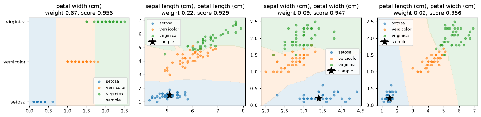
There is one panel per subspace, heaviest first: a strip plot with decision intervals for a single feature, a scatter plot with decision regions for a pair, and a 3-D scatter for three features. The title gives the weight and the individual score. sample marks the point being explained. The function returns the figure without showing it, and needs the plot extra.

Choosing the parameters

The defaults are pairs of features, at most five subspaces, complementary selection and leave-one-out scoring. The settings worth changing, with what the benchmark says about them:

Parameter	Default	When to change it
subspace_size	2	(1, 2, 3) with eight subspaces was the most accurate setting in the benchmark, 0.798 mean macro-F1 against 0.780 for five pairs, at the price of three-dimensional pictures. (1, 2) adds single-feature strips, the easiest pictures to read.
n_subspaces	5	The picture budget. Three pairs averaged 0.777 against 0.780 for five. Complementary selection may use fewer when more would not help.
max_candidates	1000	Lower it when memory or fit time matters: complementary selection stores the out-of-fold probabilities of every candidate. Above the cap, features are screened by their one-dimensional score.
n_neighbors	5	Tune it like any kNN, for example with GridSearchCV.
balance_classes	True	Weights classes equally in the selection loss, which suits macro-averaged metrics. False weights samples equally, so on imbalanced data the majority class dominates the selection.
voting	"soft"	"hard" makes each subspace cast a one-hot vote, both in selection and prediction.
cv	"loo"	Exact leave-one-out is the cheapest and needs no random split. An integer or a splitter uses k-fold out-of-fold predictions instead.
scoring	"f1_macro"	Only screens, ranks and reports subspaces; complementary selection always minimises the Brier score.
selection	"complementary"	"ranked" keeps the best individual scores, as ikNN does. selection="ranked", cv=5, max_candidates=100 reproduces version 0.1.0 up to how scores are averaged over folds.

The estimator follows the scikit-learn estimator contract, so parameters can be searched like any other:

from sklearn.model_selection import GridSearchCV

search = GridSearchCV(
    make_pipeline(StandardScaler(), SubspaceKNNClassifier()),
    {
        "subspaceknnclassifier__n_neighbors": [3, 5, 9],
        "subspaceknnclassifier__subspace_size": [2, (1, 2, 3)],
    },
    scoring="f1_macro",
)

Probabilities

predict_proba returns the weighted average of the subspaces' probabilities, and predict is its argmax, so the two always agree. Complementary selection minimises a proper scoring rule, but five-neighbour models give coarse probabilities; wrap the estimator in CalibratedClassifierCV when calibrated probabilities matter.

Limitations

• Features must be numeric; encode categorical features first, since the neighbourhood geometry depends on the encoding.
• The number of candidate subspaces grows combinatorially with the number of features. Screening by one-dimensional scores keeps it within max_candidates, but can miss features that only matter in combination.
• Complementary means complementary under probability averaging: a weak but independent signal can be left out when averaging it in would blur confident predictions. The method note explains when.
• Classification only.