Rolling Windows in Signal Processing

Rolling Window

The concept of rolling windows is deceptively simple, yet it holds significant power in signal processing and data analysis. Much like managing tasks in small portions, rolling windows allow us to break down complex datasets into manageable segments. This approach enables a range of analyses, from smoothing noisy signals to extracting critical features and performing time-frequency transformations.

In this article, we’ll explore the diverse applications of rolling windows in signal processing, covering both the underlying theory and practical implementations.

1. Technical Introduction to Rolling Windows

Understanding Rolling Windows

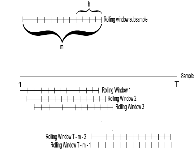
Rolling windows, also known as sliding or moving windows, are subsets of data that move sequentially across a dataset. This technique is invaluable in signal processing and time-series analysis, where temporal dependency plays a crucial role. By breaking down the dataset into smaller overlapping or non-overlapping sections, we can perform localized operations that are essential for understanding and manipulating the underlying signal characteristics.

Rolling windows are frequently used in fields such as finance, biology, and engineering to analyze sequential data. In finance, they are used to compute moving averages of stock prices, providing insights into market trends. In biological signals, rolling windows help analyze physiological data like ECG and EEG signals, enabling real-time monitoring of heart and brain activities. Engineering applications include analyzing vibration data from machinery to detect potential faults.

Formal Definition

Let’s define a discrete signal \(y[t]\) for \(t\) ranging from 0 to \(N - 1\). A rolling window of size \(n\) at a given position \(t\) consists of the segment:

\[w_t = [y[t], y[t + 1], \dots, y[t + n - 1]]\]

An operation \(O\) is applied to each window to produce a result \(M_t\):

\[M_t = O(w_t)\]

The stride \(s\) determines the movement of the window. If \(s = 1\), the windows overlap completely; if \(s = n\), the windows do not overlap at all. The choice of stride and window size depends on the specific characteristics of the data and the objectives of the analysis. For example, in high-frequency financial data, smaller strides allow for more granular insights, while in long-term climate data, larger windows may be more appropriate.

Visualization and Applications in Signal Processing

Visualizing a rolling window is akin to a conveyor belt moving across the data, processing each segment independently. This method allows for localized analysis and manipulation of the signal, enabling a variety of applications such as:

• Feature Extraction: Calculating statistical measures like mean, variance, and more sophisticated features such as entropy and skewness over different segments of the signal.
• Signal Smoothing: Reducing noise by averaging over localized segments, thus making it easier to identify the underlying trends.
• Peak and Valley Detection: Identifying significant changes within the signal, crucial for event detection in fields such as seismology and biomedical signal analysis.
• Time-Frequency Analysis: Using methods like the Short-Time Fourier Transform (STFT) to explore frequency components over time, which is essential in audio processing and radar signal analysis.

Rolling windows provide a versatile and dynamic approach to signal processing. By adjusting window size and stride, one can tailor the analysis to either focus on local variations or broader trends, making this technique a valuable tool in both exploratory data analysis and real-time processing scenarios.

2. Using Rolling Windows as Feature Extractors

Motivation

In many data-driven applications, particularly those involving machine learning, raw signals often contain excessive noise and irrelevant information. Extracting meaningful features using rolling windows can simplify the data, reduce dimensionality, and highlight patterns that are crucial for predictive modeling. This is particularly useful in fields like finance, healthcare, and environmental monitoring.

In machine learning, raw time-series data are often too complex and noisy to be directly used for modeling. Rolling windows allow us to transform these raw signals into a set of meaningful features that can improve the performance of machine learning models. For example, in anomaly detection tasks, features such as the rolling mean and standard deviation can help identify unusual patterns in the data that may indicate faults or abnormal events.

Feature Extraction Process

The process involves defining the window size \(n\) and stride \(s\), determining the features to extract, and sliding the window across the signal. Common features include:

• Mean: Provides a measure of the signal’s central tendency within each window. This feature is useful for identifying general trends in the data.
• Standard Deviation (Std): Measures the dispersion of the signal values, giving insights into the variability within each window.
• Peak-to-Peak (PtP) Distance: Indicates the range of the signal within the window, useful for capturing amplitude variations.
• Energy: Quantifies the signal’s power by summing the squares of the values. This is particularly relevant in applications like audio processing, where signal energy can indicate the presence of sound.
• Zero-Crossing Rate: Useful in frequency analysis, indicating the rate at which the signal changes sign. It is commonly used in speech processing to distinguish between voiced and unvoiced sounds.

Selecting the right window size and stride is critical. Smaller windows capture finer details but are more sensitive to noise, while larger windows provide a smoothed view of the signal at the cost of losing some granular information.

Example Use Case

Consider a dataset comprising multiple sensor readings. By applying rolling windows to extract features, we can convert each signal into a set of meaningful attributes suitable for machine learning models like logistic regression or support vector machines. This transformation enhances the model’s ability to discern patterns, leading to more accurate predictions. For instance, in wearable sensor data, rolling window features can help classify different physical activities such as walking, running, and sitting by capturing the dynamic characteristics of movement.

3. Smoothing Signals with Rolling Windows

The Need for Smoothing

Real-world signals are often contaminated with noise, making it challenging to identify underlying trends and patterns. Smoothing is a technique used to mitigate this issue, thereby clarifying the signal’s inherent structure. Common applications include biomedical signal processing, where noise reduction is crucial for interpreting heart and brain activity, and financial data analysis, where it helps identify market trends.

Noise can arise from various sources, such as sensor inaccuracies, environmental factors, or inherent variability in the process being measured. In biomedical applications, for example, signals such as ECG and EEG are often contaminated with noise from muscle activity or external electrical sources. Smoothing helps reduce these unwanted variations, making it easier to detect critical events like heartbeats or brain waves.

Moving Average Filter

One of the simplest and most commonly used smoothing techniques is the moving average filter. By replacing each data point with the average of its neighboring points within a window, the moving average filter effectively reduces high-frequency noise. However, this approach has limitations, such as potential blurring of sharp features and the introduction of phase shifts.

The moving average filter is particularly effective when the goal is to reduce random noise while preserving the general shape of the signal. For example, in financial data analysis, a moving average of stock prices can help identify long-term trends by smoothing out short-term fluctuations. However, care must be taken when using this filter, as it can introduce a lag, making it less suitable for real-time analysis where immediate response to changes is required.

Savitzky-Golay Filter

The Savitzky-Golay filter offers a more sophisticated approach by fitting a low-degree polynomial to the data points within each window. This method smooths the signal while preserving its key characteristics, such as peak height and width, making it more suitable for applications where retaining signal features is essential.

The mathematical foundation of the Savitzky-Golay filter involves fitting a polynomial of degree \(p\) to each window:

\[\min \sum_{i=-k}^{k} \left(y_{t+i} - \sum_{j=0}^{p} a_j i^j \right)^2\]

This minimization ensures that the polynomial approximates the underlying trend of the signal within each window, leading to an efficient noise reduction mechanism that does not distort important features. This is particularly useful in spectroscopic analysis, where the goal is to smooth the data while preserving the shape and width of spectral peaks.

4. Peak and Valley Detection Using Rolling Windows

Importance of Peak Detection

Detecting peaks and valleys is vital in many signal processing applications, such as identifying heartbeats in ECG signals, detecting stock market highs and lows, and monitoring environmental events. Rolling windows provide a localized view of the signal, making it possible to detect these critical points with precision.

In the context of biomedical signals, peak detection is essential for analyzing heart rate variability and other physiological parameters. For instance, the detection of R-peaks in ECG signals allows for the computation of heart rate, a key indicator of cardiovascular health. Similarly, in seismic signal analysis, identifying peaks can help detect and characterize earthquake events.

Rolling Window Approach

By using rolling windows, we compute local statistics (such as the mean and standard deviation) and identify points that significantly deviate from these statistics. This approach allows us to set thresholds that adapt to the signal’s local behavior, making peak detection more robust to noise and variability.

For each point \(x_t\), we determine if it is a peak by comparing it to the local mean \(\mu_{t-1}\) and standard deviation \(\sigma_{t-1}\). If \(x_t > \mu_{t-1} + \theta \sigma_{t-1}\), it is identified as a positive peak; if \(x_t < \mu_{t-1} - \theta \sigma_{t-1}\), it is a negative peak.

This method is particularly useful in scenarios where the signal’s characteristics vary over time. By using rolling windows, we adapt to these changes, allowing for more accurate peak detection in dynamic environments. For example, in stock market analysis, this approach can help identify local maxima and minima, providing insights into market cycles and aiding in trading decisions.

5. Applying Rolling Windows for Fourier Transform

Limitations of Standard Fourier Transform

The standard Fourier Transform (FT) assumes that the signal’s frequency components remain constant over time, which is not the case for many real-world signals. Signals such as speech or music are non-stationary, meaning their frequency content changes over time.

For instance, consider an audio signal where the pitch varies over time. A standard Fourier Transform would provide the overall frequency content, but it would not reveal how the frequencies change as the signal progresses. This limitation makes it difficult to analyze signals with transient components, such as musical notes or speech phonemes, where the frequency content is dynamic.

Short-Time Fourier Transform (STFT)

The Short-Time Fourier Transform (STFT) addresses this limitation by applying the FT to short, overlapping segments of the signal. This allows us to analyze how the signal’s frequency content evolves, providing a time-frequency representation that is crucial for understanding non-stationary signals.

In STFT, the signal is divided into overlapping windows, each multiplied by a window function (e.g., Hann window) to reduce spectral leakage. The Fourier Transform is then computed for each segment, resulting in a spectrogram that visualizes the signal’s frequency components over time.

The STFT is widely used in applications like speech processing, music analysis, and biomedical signal analysis. For example, in speech processing, STFT helps analyze the frequency content of phonemes, aiding in tasks such as speech recognition and speaker identification. In biomedical signal analysis, STFT can reveal how the frequency content of EEG signals changes over time, providing insights into brain activity and helping diagnose neurological conditions.

Appendix: Mathematics and Code

A. Technical Definitions

Rolling Window Extraction

Given a signal \(y[t]\) and window size \(n\), the window at position \(t\) is defined as:

\[w_t = [y[t], y[t + 1], \dots, y[t + n - 1]]\]

An operation \(O\) applied to each window yields:

\[M_t = O(w_t)\]

Stride Movement

The stride \(s\) defines the movement of the window across the signal. For stride \(s\), the next window starts at \(t + s\). Choosing the appropriate stride is crucial; smaller strides result in more overlapping windows, providing more data points but increasing computational cost.

B. Feature Extraction Code

import numpy as np
import pandas as pd

def extract_features(signal, window_size, stride):
    features = {'mean': [], 'std': [], 'ptp': [], 'energy': []}
    indices = range(0, len(signal) - window_size + 1, stride)
    for i in indices:
        window = signal[i:i+window_size]
        features['mean'].append(np.mean(window))
        features['std'].append(np.std(window))
        features['ptp'].append(np.ptp(window))
        features['energy'].append(np.sum(window**2))
    return pd.DataFrame(features)

# Example usage
signal = np.random.randn(1000)
window_size = 50
stride = 25
features_df = extract_features(signal, window_size, stride)
print(features_df.head())

This code snippet demonstrates how to extract features from a signal using rolling windows. By selecting an appropriate window size and stride, the function computes mean, standard deviation, peak-to-peak distance, and energy for each window. These features can then be used in machine learning models for tasks such as classification, regression, or anomaly detection.

C. Savitzky-Golay Filter Mathematics

The Savitzky-Golay filter smooths data by fitting successive sub-sets of adjacent data points with a low-degree polynomial using a least-squares method. The polynomial order and window size are crucial parameters that determine the filter’s behavior:

\[\min \sum_{i=-k}^{k} \left( y_{t+i} - \sum_{j=0}^{p} a_j i^j \right)^2\]

Where:

• \(k = \frac{n - 1}{2}\) is half the window size.
• \(p\) is the polynomial order.
• \(a_j\) are the polynomial coefficients to be determined.

Convolution Coefficients

The filter can be efficiently implemented as a convolution operation using precomputed coefficients. These coefficients depend on the window size and polynomial order.

D. Peak Detection Algorithm

Detection Criteria

For each point \(x_t\):

• Positive Peak: \(x_t > \mu_{t-1} + \theta \sigma_{t-1}\)
• Negative Peak: \(x_t < \mu_{t-1} - \theta \sigma_{t-1}\)

Where \(\mu_{t-1}\) and \(\sigma_{t-1}\) are the mean and standard deviation of the previous window, and \(\theta\) is the threshold in terms of standard deviations.

Influence Update

When a peak is detected:

• With Influence: Adjust the signal value.
• Without Influence: Do not include \(x_t\) in future calculations.

E. Short-Time Fourier Transform Code

from scipy.signal import stft
import numpy as np
import matplotlib.pyplot as plt

# Signal parameters
fs = 1000  # Sampling frequency
t = np.arange(0, 5, 1/fs)

# Signal with multiple frequency components at different times
signal = np.zeros_like(t)
signal[(t >= 0) & (t < 1)] = np.sin(2 * np.pi * 50 * t[(t >= 0) & (t < 1)])
signal[(t >= 1) & (t < 2)] = np.sin(2 * np.pi * 100 * t[(t >= 1) & (t < 2)])
signal[(t >= 2) & (t < 3)] = np.sin(2 * np.pi * 150 * t[(t >= 2) & (t < 3)])
signal[(t >= 3) & (t < 4)] = np.sin(2 * np.pi * 200 * t[(t >= 3) & (t < 4)])
signal[(t >= 4) & (t <= 5)] = np.sin(2 * np.pi * 250 * t[(t >= 4) & (t <= 5)])

# Compute STFT
f, t_stft, Zxx = stft(signal, fs=fs, window='hann', nperseg=256, noverlap=128)

# Plot spectrogram
plt.figure(figsize=(12, 6))
plt.pcolormesh(t_stft, f, np.abs(Zxx), shading='gouraud')
plt.title('STFT Spectrogram of Signal with Time-Varying Frequencies')
plt.ylabel('Frequency [Hz]')
plt.xlabel('Time [sec]')
plt.ylim(0, 300)
plt.colorbar(label='Magnitude')
plt.show()

This code demonstrates how to perform the Short-Time Fourier Transform on a signal. By computing the STFT, we obtain a spectrogram that shows how the signal’s frequency content changes over time, making it possible to analyze non-stationary signals in detail.

References

Books

1. Digital Signal Processing: A Practical Guide for Engineers and Scientists by Steven W. Smith
   • This book provides a comprehensive introduction to digital signal processing (DSP) concepts, including practical applications and techniques like rolling windows, filtering, and Fourier analysis.
2. Time Series Analysis and Its Applications by Robert H. Shumway and David S. Stoffer
   • A detailed guide to time-series analysis, including concepts like moving averages, smoothing techniques, and feature extraction in time-series data.
3. Pattern Recognition and Machine Learning by Christopher M. Bishop
   • Covers machine learning techniques that can benefit from rolling window feature extraction in time-series data, such as classification and anomaly detection.
4. Applied Time Series Analysis by Terence C. Mills
   • An introduction to time-series analysis with a focus on practical applications, including the use of rolling windows for analysis and forecasting.
5. Numerical Recipes: The Art of Scientific Computing by William H. Press et al.
   • Offers a wealth of numerical methods, including those relevant to rolling windows, signal processing, and data smoothing.

Research Papers

1. “A Tutorial on Hidden Markov Models and Selected Applications in Speech Recognition” by Lawrence R. Rabiner
   • While focused on Hidden Markov Models, this paper provides insights into signal processing techniques such as short-time analysis and feature extraction using rolling windows.
2. “Rolling Analysis of Time Series” by Alexandros C. Trindade
   • A comprehensive exploration of rolling analysis methods in time series, including statistical measures and practical applications.
3. “Feature Extraction and Classification of EEG Signals Using Neural Networks” by Sami F. Atoui et al.
   • Demonstrates the use of rolling windows for extracting features from EEG signals, highlighting their application in biomedical signal processing.
4. “Anomaly Detection in Time Series: An Introduction with NASA Data” by R. J. Hyndman et al.
   • Discusses time-series anomaly detection using rolling windows, with practical examples applied to NASA datasets.

Online Courses and Tutorials

1. Digital Signal Processing Specialization on Coursera
   • A series of courses that cover fundamental concepts in DSP, including filtering, Fourier transforms, and practical signal processing using rolling windows.
   • Link
2. Time Series Analysis with Python by DataCamp
   • An interactive course focusing on time-series analysis in Python, including rolling window calculations and feature extraction.
   • Link
3. Signal Processing Using Python (SciPy) by SciPy.org
   • A collection of tutorials and documentation covering signal processing in Python, including smoothing, filtering, and rolling window operations.
   • Link

Academic Journals

1. IEEE Transactions on Signal Processing
   • Publishes articles on the theory, implementation, and application of signal processing, including advanced topics related to rolling windows and time-series analysis.
   • Link
2. Journal of Time Series Analysis
   • A journal that focuses on new and original research in the area of time-series analysis, including practical applications of rolling windows in various fields.
   • Link

Blogs and Articles

1. “A Comprehensive Guide to Time Series Analysis and Forecasting” by Towards Data Science
   • An overview of time-series analysis techniques, including moving averages and feature extraction using rolling windows.
   • Link
2. “Signal Processing with Python - Analyzing Audio Signals with STFT” by Real Python
   • A practical guide on using Short-Time Fourier Transform (STFT) in Python for analyzing audio signals.
   • Link
3. “Rolling Window Analysis of Time Series in Python” by Analytics Vidhya
   • A tutorial on how to perform rolling window analysis in Python, including implementation examples.
   • Link

Software and Toolkits

1. SciPy
   • A Python library for scientific computing that includes modules for signal processing, such as filtering, STFT, and other techniques relevant to rolling windows.
   • Link
2. NumPy
   • A fundamental package for numerical computation in Python that provides efficient implementations of array operations, including rolling windows.
   • Link
3. pandas
   • A Python library for data manipulation and analysis, offering built-in support for rolling window operations on time-series data.
   • Link

Check out Data Science Books on Amazon