Applying R Functions on Rolling Windows Using the runner Package
runner Package
Overview of the runner Package
The runner package provides flexible and powerful functions to apply any R function over running (or rolling) windows of data. It stands out from other rolling window libraries by supporting any input/output types and offering full control over window size and lags, making it highly versatile for various use cases like time series analysis, cumulative operations, and sliding windows.
The core function in this package, runner::runner(), allows users to define window size (k), lag (lag), and an index (idx) to customize how the window moves through the dataset. This function can handle complex, real-world data with missing values, non-sequential time indices, and variable window sizes. The runner package offers a wide range of windowing types and customizations, making it a powerful tool for rolling computations.
Types of Rolling Windows in runner
The runner package supports several types of rolling windows, each serving different use cases, from simple cumulative sums to complex time-based windows. Here, we discuss the most common types of windows supported by the package.
1. Cumulative Windows
A cumulative window starts from the first element and expands to include each subsequent element. This type is similar to base::cumsum, where each value in the window contains all elements up to the current position.
Example of a simple cumulative window:
library(runner)

# Cumulative windows on a numeric sequence
runner(1:15)

# Cumulative sum
runner(1:15, f = sum)

# Concatenating characters in cumulative windows
runner(letters[1:15], f = paste, collapse = " > ")
Cumulative windows are useful for running totals, aggregations, or growing-window computations where each window includes all previous observations.
2. Constant Sliding Windows
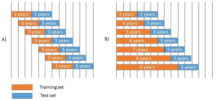
Sliding windows (also known as rolling or moving windows) move over the dataset by a fixed size k, producing windows of equal length, except at the start. These windows are useful for calculating rolling statistics like moving averages or running linear models.
The following diagram illustrates a rolling window of size k = 4 over a dataset of 15 elements. Each window contains 4 elements (except the first few):
# Sliding window: Summing over a 4-element window
runner(1:15, k = 4, f = sum)

# Rolling regression slope using `lm`
df <- data.frame(a = 1:15, b = 3 * 1:15 + rnorm(15))
runner(df, k = 5, f = function(x) {
  model <- lm(b ~ a, data = x)
  coefficients(model)["a"]
})
Sliding windows are often used in time series analysis, such as calculating rolling averages, volatility, or regressions over a constant window size.
3. Windows Based on Date or Time
For datasets where the index represents dates or time (e.g., financial data, sensor readings), the window size can vary based on the time gaps between observations. By specifying the idx argument, one can define windows based on actual time intervals instead of sequential indices.
Example of a date-based window:
idx <- c(4, 6, 7, 13, 17, 18, 18, 21, 27, 31, 37, 42, 44, 47, 48)

# Mean calculation for a 5-day window with a lag of 1 day
runner(x = idx, k = 5, lag = 1, idx = idx, f = mean)

# Using date sequences
runner(x = idx, k = "5 days", lag = 1, idx = Sys.Date() + idx, f = mean)
This is particularly useful when dealing with irregular time series, where observations may be missing due to weekends, holidays, or other reasons, and windows should reflect meaningful time spans rather than fixed counts.
4. Custom Windows with at
The at argument allows you to specify custom indices where the function should be applied. Instead of calculating the function at every possible window position, at provides control over specific points of interest.
idx <- c(4, 6, 7, 13, 17, 18, 18, 21, 27, 31, 37, 42, 44, 47, 48)

# Apply mean function at specific indices
runner(x = 1:15, k = 5, lag = 1, idx = idx, at = c(18, 27, 48, 31), f = mean)

# Use a 4-month interval
idx_date <- seq(Sys.Date(), Sys.Date() + 365, by = "1 month")
runner(x = 0:12, idx = idx_date, at = "4 months")
This feature is particularly useful for long datasets where calculating at every index would be inefficient, or when specific periodic points are of interest.
5. Flexible Window Sizes and Lags
The runner package allows complete flexibility in specifying window sizes (k) and lags (lag). Both can be integers or time intervals. If a constant window size and lag are not sufficient, they can be provided as vectors, allowing for variable window sizes and lags across different parts of the dataset.
Example of varying k and lag:
runner(x = 1:10,
       lag = c(-1, 2, -1, -2, 0, 0, 5, -5, -2, -3),
       k = c(0, 1, 1, 1, 1, 5, 5, 5, 5, 5),
       f = paste, collapse = ",")
This flexibility supports complex use cases where windows of different sizes or with different lags are needed for different parts of the dataset, such as in irregularly spaced time series or datasets with varying data frequencies.
6. Handling NA Values with na_pad
By default, runner handles incomplete windows by calculating the function for any available data. However, when you need to return NA for incomplete windows (e.g., when not enough observations are available to fill the window), you can set na_pad = TRUE.
runner(x = 1:15, k = 5, lag = 1, idx = idx, at = c(4, 18, 48, 51), na_pad = TRUE, f = mean)
This behavior ensures more robust handling of missing data, especially in time series where you may want to avoid biased calculations from incomplete windows.
7. Applying runner on Data Frames
The runner function can also be applied to data.frame objects. This is especially useful for running statistical models like regressions on subsets of the data.
x <- cumsum(rnorm(40))
y <- 3 * x + rnorm(40)
date <- Sys.Date() + cumsum(sample(1:3, 40, replace = TRUE))
group <- rep(c("a", "b"), 20)
df <- data.frame(date, group, y, x)

# Calculate the slope of `y ~ x` over a rolling window
slope <- runner(df, f = function(x) coefficients(lm(y ~ x, data = x))[2])

plot(slope)
This example shows how to calculate the rolling slope of a regression model (y ~ x) as more observations become available.
8. runner with dplyr and ggplot2
The runner package integrates seamlessly with dplyr and can be used for grouped operations without the need for group_modify(). The following example shows how to compute a rolling beta coefficient for each group in a dataset using dplyr.
library(dplyr)
library(ggplot2)

summ <- df %>%
  group_by(group) %>%
  mutate(
    cumulative_mse = runner(
      x = .,
      k = "20 days",
      idx = "date",
      f = function(x) coefficients(lm(y ~ x, data = x))[2]
    )
  )

# Plot results using `ggplot2`
summ %>%
  ggplot(aes(x = date, y = cumulative_mse, group = group, color = group)) +
  geom_line()
This example shows how to use runner within a dplyr pipeline to compute and visualize rolling regression coefficients over time for different groups.
9. Parallel Processing
For larger datasets, runner supports parallel computation. This can speed up the process when applying complex functions over many rolling windows.
library(parallel)

numCores <- detectCores()
cl <- makeForkCluster(numCores)

runner(x = df, k = 10, idx = "date", f = function(x) sum(x$x), cl = cl)

stopCluster(cl)
Using parallel mode can significantly improve performance, particularly for CPU-intensive computations. However, parallel processing also introduces overhead, so it’s essential to test whether parallelization is beneficial for your specific case.
Built-in Optimized Functions
The runner package includes several optimized functions for common rolling computations to improve performance:
- Aggregating functions:
length_run,min_run,max_run,minmax_run,sum_run,mean_run,streak_run - Utility functions:
fill_run,lag_run,which_run
These built-in functions are designed for speed and efficiency and can handle large datasets efficiently.
# Example of using `sum_run` for optimized rolling sum
runner(1:1000, f = sum_run)
These functions can be used when speed is critical, and they offer a convenient shorthand for common rolling operations.


