Probability Integral Transform: Theory and Applications
Introduction
What is the Probability Integral Transform?
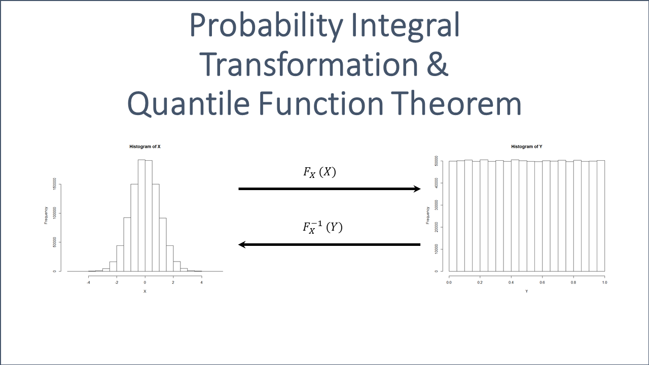
The Probability Integral Transform is a fundamental concept in statistics and probability theory. It enables the conversion of a random variable with any continuous distribution into a random variable with a uniform distribution on the interval \([0, 1]\).
Definition and Basic Explanation
Given a continuous random variable \(X\) with a cumulative distribution function (CDF) \(F_X(x)\), the transform states that the random variable \(Y = F_X(X)\) follows a uniform distribution on the interval \([0, 1]\). This can be expressed mathematically as:
\[Y = F_X(X)\]where:
- \(X\) is a continuous random variable.
- \(F_X(x)\) is the CDF of \(X\).
- \(Y\) is a new random variable that is uniformly distributed over \([0, 1]\).
To understand why this transformation works, consider the properties of the CDF. The CDF, \(F_X(x)\), of a random variable \(X\) is defined as:
\[F_X(x) = P(X \leq x)\]This function \(F_X(x)\) maps values of \(X\) to probabilities in the range \([0, 1]\). Since \(F_X(x)\) is a monotonically increasing function that spans from 0 to 1 as \(x\) goes from \(-\infty\) to \(\infty\), applying \(F_X\) to \(X\) standardizes these probabilities, transforming \(X\) into a new random variable \(Y\) that is uniformly distributed between 0 and 1.
Importance in Statistics and Probability Theory
The Probability Integral Transform is crucial for several reasons:
-
Simplification and Standardization: By transforming any continuous random variable into a uniform distribution, it simplifies the process of working with different distributions. This standardization is particularly useful in theoretical derivations and practical applications.
-
Foundation for Further Analysis: Many statistical methods and tests rely on the uniformity of transformed data. For example, goodness of fit tests often use the Probability Integral Transform to compare observed data with expected distributions.
-
Enabling Complex Models: The transform is a key tool in constructing copulas, which are functions used to describe the dependence structure between random variables. This is particularly useful in multivariate analysis where understanding the relationship between variables is crucial.
-
Improving Simulation and Random Sampling: In Monte Carlo simulations and random sample generation, the Probability Integral Transform allows for the creation of samples from any desired distribution. By first generating uniform random variables and then applying the inverse CDF of the target distribution, we can simulate data that follows complex distributions.
Understanding the Probability Integral Transform provides a powerful toolset for both theoretical explorations and practical applications in statistics and probability. It serves as a bridge between various distributions, facilitating analysis, testing, and simulation in a standardized manner.
Why Does It Work?
The Probability Integral Transform works due to the inherent properties of cumulative distribution functions (CDFs). The transformation of any continuous random variable into a uniformly distributed random variable relies on the mathematical basis and behavior of CDFs.
Explanation of the Mathematical Basis
To understand why the Probability Integral Transform works, let’s start with the definition of a cumulative distribution function (CDF). For a continuous random variable %%X\(with CDF\)F_X(x)$$, the CDF is defined as:
\[F_X(x) = P(X \leq x)\]This equation states that \(F_X(x)\) is the probability that the random variable \(X\) takes on a value less than or equal to \(x\).
Now, consider the transformed variable \(Y\):
\[Y = F_X(X)\]Here, \(Y\) is a new random variable created by applying the CDF of \(X\) to itself. To show that \(Y\) is uniformly distributed over the interval \([0, 1]\), we need to demonstrate that the CDF of \(Y\), denoted as \(F_Y(y)\), follows a uniform distribution.
The CDF of \(Y\) is given by:
\[F_Y(y) = P(Y \leq y) = P(F_X(X) \leq y)\]Since \(F_X\) is a monotonically increasing function, we can invert it to find \(X\):
\[P(F_X(X) \leq y) = P(X \leq F_X^{-1}(y))\]By the definition of the CDF \(F_X\), we have:
\[P(X \leq F_X^{-1}(y)) = F_X(F_X^{-1}(y)) = y\]Therefore:
\[F_Y(y) = y\]This shows that the CDF of \(Y\) is \(y\) for \(y\) in the interval \([0, 1]\), which is the CDF of a uniform distribution on \([0, 1]\). Thus, \(Y\) is uniformly distributed.
Role of Cumulative Distribution Functions (CDFs)
The role of CDFs is central to the Probability Integral Transform. The CDF \(F_X(x)\) encapsulates all the probabilistic information about the random variable \(X\). When we apply \(F_X\) to \(X\), we leverage this information to standardize the variable into a uniform distribution.
Key properties of CDFs that make the Probability Integral Transform work include:
-
Monotonicity: CDFs are monotonically increasing functions. This means that as the value of \(X\) increases, \(F_X(x)\) also increases. This property ensures that the transformation \(Y = F_X(X)\) is well-defined and maps \(X\) to the interval \([0, 1]\).
-
Range: The range of a CDF is always between 0 and 1, inclusive. This range matches the desired uniform distribution range for the transformed variable \(Y\).
-
Invertibility: For continuous random variables, the CDF \(F_X\) is invertible. This allows us to map back from the uniform distribution to the original distribution if needed, using the inverse CDF \(F_X^{-1}\).
-
Probabilistic Interpretation: The CDF \(F_X(x)\) gives the probability that \(X\) is less than or equal to \(x\). This probabilistic interpretation is preserved in the transform, making \(Y = F_X(X)\) a probabilistically meaningful transformation.
The Probability Integral Transform leverages these properties of CDFs to convert any continuous random variable into a uniformly distributed variable, facilitating various statistical methods and analyses.
Practical Applications
Copula Construction
Copulas are powerful tools in statistics that allow for modeling and analyzing the dependence structure between multiple random variables. They are particularly useful in multivariate analysis, finance, risk management, and many other fields where understanding the relationships between variables is crucial.
Description of Copulas
A copula is a function that links univariate marginal distribution functions to form a multivariate distribution function. Essentially, it describes the dependency structure between random variables, separate from their marginal distributions. Formally, a copula \(C\) is a multivariate cumulative distribution function with uniform marginals on the interval \([0, 1]\).
The Sklar’s Theorem is fundamental in the theory of copulas. It states that for any multivariate cumulative distribution function \(F\) with marginals \(F_1, F_2, \ldots, F_n\), there exists a copula \(C\) such that:
\[F(x_1, x_2, \ldots, x_n) = C(F_1(x_1), F_2(x_2), \ldots, F_n(x_n))\]Conversely, if \(C\) is a copula and \(F_1, F_2, \ldots, F_n\) are cumulative distribution functions, then \(F\) defined above is a joint cumulative distribution function with marginals \(F_1, F_2, \ldots, F_n\).
How the Transform Aids in Creating Copulas
The Probability Integral Transform plays a crucial role in constructing copulas. Here’s how it aids in the process:
-
Uniform Marginals: The Probability Integral Transform converts any continuous random variable into a uniform random variable on the interval \([0, 1]\). This is essential for copula construction, as copulas require uniform marginals.
-
Standardizing Marginal Distributions: Given random variables \(X_1, X_2, \ldots, X_n\) with continuous marginal distribution functions \(F_{X1}, F_{X2}, \ldots, F_{Xn}\), we can transform these variables using their respective CDFs to obtain uniform variables:
\[U_i = F_{Xi}(X_i)\]for \(i = 1, 2, \ldots, n\). Each \(U_i\) is uniformly distributed over \([0, 1]\).
-
Constructing the Copula: With the transformed variables \(U_1, U_2, \ldots, U_n\), we can now construct a copula \(C\). The copula captures the dependence structure between the original random variables \(X_1, X_2, \ldots, X_n\):
\[C(u_1, u_2, \ldots, u_n) = F(F_{X1}^{-1}(u_1), F_{X2}^{-1}(u_2), \ldots, F_{Xn}^{-1}(u_n))\]Here, \(F\) is the joint cumulative distribution function of the original random variables, and \(F_{Xi}^{-1}\) are the inverse CDFs (quantile functions) of the marginals.
-
Flexibility in Modeling Dependence: By separating the marginal distributions from the dependence structure, copulas provide flexibility in modeling. We can choose appropriate marginal distributions for the individual variables and a copula that best describes their dependence.
Probability Integral Transform is essential for constructing copulas because it standardizes the marginal distributions of random variables to a uniform scale. This standardization is a prerequisite for applying Sklar’s Theorem and effectively modeling the dependence structure between variables using copulas.
Goodness of Fit Tests
Goodness of fit tests are essential statistical procedures used to determine how well a statistical model fits a set of observations. They play a crucial role in model validation, ensuring that the model accurately represents the underlying data.
Importance of Goodness of Fit
Goodness of fit tests serve several critical purposes:
- Model Validation: They help validate the assumptions made by a statistical model. If a model fits well, it suggests that the assumptions are reasonable and the model is likely to be accurate in predictions and interpretations.
- Comparison of Models: These tests allow for the comparison of different models. By assessing which model provides a better fit to the data, researchers can select the most appropriate model for their analysis.
- Detection of Anomalies: Goodness of fit tests can identify deviations from expected patterns, highlighting potential anomalies or areas where the model may be failing to capture important aspects of the data.
- Improving Model Reliability: Regularly applying goodness of fit tests helps in refining models, leading to improved reliability and robustness in statistical analysis and predictions.
Using the Transform to Assess Model Fit
The Probability Integral Transform is a powerful tool for assessing the goodness of fit of a model. Here’s how it can be applied:
-
Transformation to Uniform Distribution: Given a model with a cumulative distribution function (CDF) \(F\) and observed data points \(x_1, x_2, \ldots, x_n\), we can transform these observations using the model’s CDF:
\[y_i = F(x_i)\]for \(i = 1, 2, \ldots, n\). If the model fits the data well, the transformed values \(y_i\) should follow a uniform distribution on the interval \([0, 1]\).
-
Visual Assessment: One simple method to assess the goodness of fit is through visual tools like Q-Q (quantile-quantile) plots. By plotting the quantiles of the transformed data against the quantiles of a uniform distribution, we can visually inspect whether the points lie approximately along a 45-degree line, indicating a good fit.
- Formal Statistical Tests: Several formal statistical tests can be applied to the transformed data to assess uniformity. Some of these tests include:
- Kolmogorov-Smirnov Test: Compares the empirical distribution function of the transformed data with the uniform distribution.
- Anderson-Darling Test: A more sensitive test that gives more weight to the tails of the distribution.
- Cramér-von Mises Criterion: Assesses the discrepancy between the empirical and theoretical distribution functions.
-
Residual Analysis: In regression models, the Probability Integral Transform can be applied to the residuals (differences between observed and predicted values). By transforming the residuals and assessing their uniformity, we can determine if the residuals behave as expected under the model assumptions.
- Histogram and Density Plots: Creating histograms or density plots of the transformed data and comparing them to the uniform distribution can provide a visual check for goodness of fit. Deviations from the expected uniform shape can indicate areas where the model may not be fitting well.
The Probability Integral Transform is a valuable tool for goodness of fit tests, allowing for both visual and formal assessments of how well a model represents the data. By transforming data using the model’s CDF and evaluating the resulting uniformity, researchers can gain insights into the accuracy and reliability of their statistical models.
Monte Carlo Simulations
Monte Carlo simulations are a class of computational algorithms that rely on repeated random sampling to obtain numerical results. These methods are used to model phenomena with significant uncertainty in inputs and outputs, making them invaluable in fields such as finance, engineering, and physical sciences.
Overview of Monte Carlo Methods
Monte Carlo methods involve the following key steps:
- Random Sampling: Generate random inputs from specified probability distributions.
- Model Evaluation: Use these random inputs to perform a series of experiments or simulations.
- Aggregation of Results: Collect and aggregate the results of these experiments to approximate the desired quantity.
The power of Monte Carlo methods lies in their ability to handle complex, multidimensional problems where analytical solutions are not feasible. They provide a way to estimate the distribution of outcomes and understand the impact of uncertainty in model inputs.
Application of the Transform in Simulations
The Probability Integral Transform is crucial in Monte Carlo simulations for generating random samples from any desired probability distribution. Here’s how it can be applied:
-
Generating Uniform Random Variables: Start by generating random variables \(U\) that are uniformly distributed over the interval \([0, 1]\). This is straightforward, as most programming languages and statistical software have built-in functions for generating uniform random numbers.
-
Transforming to Desired Distribution: To transform these uniform random variables into samples from a desired distribution with cumulative distribution function (CDF) \(F\), apply the inverse CDF (also known as the quantile function) of the target distribution:
\[X = F^{-1}(U)\]Here, \(X\) is a random variable with the desired distribution. The inverse CDF \(F^{-1}\) maps uniform random variables to the distribution of \(X\).
For example, to generate samples from an exponential distribution with rate parameter \(\lambda\), use the inverse CDF of the exponential distribution:
\[X = -\frac{1}{\lambda} \ln(1 - U)\] -
Complex Distributions: For more complex distributions, numerical methods or approximations of the inverse CDF may be used. The Probability Integral Transform ensures that the samples follow the target distribution accurately.
-
Example: Estimating π: A classic example of Monte Carlo simulation is estimating the value of π. By randomly sampling points in a square and counting the number that fall inside a quarter circle, the ratio of the points inside the circle to the total points approximates π/4. This method relies on uniform random sampling within the square.
-
Variance Reduction Techniques: The Probability Integral Transform can be combined with variance reduction techniques, such as importance sampling or stratified sampling, to improve the efficiency and accuracy of Monte Carlo simulations.
- Importance Sampling: Adjusts the sampling distribution to focus on important regions of the input space, improving the estimation accuracy for rare events.
- Stratified Sampling: Divides the input space into strata and samples from each stratum to ensure better coverage and reduce variance.
-
Application in Finance: In financial modeling, Monte Carlo simulations are used to estimate the value of complex derivatives, assess risk, and optimize portfolios. By generating random samples from the distribution of asset returns, the Probability Integral Transform ensures accurate modeling of uncertainties and dependencies.
Probability Integral Transform is essential in Monte Carlo simulations for transforming uniform random variables into samples from any desired distribution. This capability allows for flexible and accurate modeling of complex systems, making Monte Carlo methods a powerful tool in various applications.
Hypothesis Testing
Hypothesis testing is a fundamental method in statistics used to make inferences about populations based on sample data. It involves formulating a hypothesis, collecting data, and then determining whether the data provide sufficient evidence to reject the hypothesis.
Role of Hypothesis Testing in Statistics
Hypothesis testing plays several critical roles in statistical analysis:
- Decision Making: It provides a structured framework for making decisions about the properties of populations. By testing hypotheses, researchers can make informed decisions based on sample data.
- Validation of Theories: Hypothesis tests are used to validate or refute theoretical models. This is crucial in scientific research where theories need empirical validation.
- Quality Control: In industrial applications, hypothesis testing is used to monitor processes and ensure quality standards are met.
- Policy Making: In fields like economics and social sciences, hypothesis tests guide policy decisions by providing evidence-based conclusions.
Standardizing Data with the Transform for Better Testing
The Probability Integral Transform can enhance hypothesis testing by standardizing data, making it easier to apply statistical tests and interpret results. Here’s how it works:
-
Transforming Data to Uniform Distribution: Given a random variable \(X\) with CDF \(F_X(x)\), the Probability Integral Transform converts \(X\) into a new random variable \(Y\) that is uniformly distributed on \([0, 1]\):
\[Y = F_X(X)\]This standardization simplifies the comparison of data to theoretical distributions.
-
Simplifying Test Assumptions: Many statistical tests assume that the data follow a specific distribution, often the normal distribution. By transforming data using the Probability Integral Transform, we can ensure the transformed data meet these assumptions more closely. For instance, the Kolmogorov-Smirnov test compares an empirical distribution to a uniform distribution, making it directly applicable to the transformed data.
- Uniformity and Hypothesis Testing: When applying the Probability Integral Transform, the transformed data \(Y\) should follow a uniform distribution if the null hypothesis holds. This uniformity can be tested using various statistical tests:
- Kolmogorov-Smirnov Test: Compares the empirical distribution of the transformed data to a uniform distribution to assess goodness of fit.
- Chi-Square Test: Can be used on binned transformed data to test for uniformity.
- Anderson-Darling Test: A more sensitive test that gives more weight to the tails of the distribution.
-
Transforming Back: If needed, the inverse CDF \(F_X^{-1}(y)\) can be used to transform the uniform data back to the original distribution for interpretation or further analysis.
-
Example in Regression Analysis: In regression models, the Probability Integral Transform can be applied to the residuals to test for normality. If the residuals are transformed and shown to be uniformly distributed, it indicates that the residuals follow the expected distribution under the null hypothesis of no systematic deviations.
- Improving Test Power: Standardizing data using the Probability Integral Transform can improve the power of statistical tests. By ensuring the data meet the test assumptions more closely, the tests are more likely to detect true effects when they exist.
The Probability Integral Transform is a valuable tool in hypothesis testing for standardizing data, simplifying assumptions, and improving the interpretability and power of statistical tests. By transforming data to a uniform distribution, it facilitates more accurate and reliable hypothesis testing in various statistical applications.
Generation of Random Samples
Generating random samples from a specified distribution is a common task in statistics and simulation. These samples are used in various applications, including simulations, bootstrapping, and probabilistic modeling.
Methods for Generating Random Samples
There are several methods for generating random samples from a desired probability distribution:
- Inverse Transform Sampling: This method involves generating uniform random variables and then applying the inverse CDF (quantile function) of the target distribution. It is particularly useful for distributions where the inverse CDF can be computed efficiently.
- Rejection Sampling: This technique generates candidate samples from an easy-to-sample distribution and then accepts or rejects each sample based on a criterion that involves the target distribution. It is useful for complex distributions where direct sampling is difficult.
- Metropolis-Hastings Algorithm: A Markov Chain Monte Carlo (MCMC) method that generates samples by constructing a Markov chain that has the desired distribution as its equilibrium distribution. It is widely used for sampling from high-dimensional distributions.
- Gibbs Sampling: Another MCMC method that generates samples from the joint distribution of multiple variables by iteratively sampling from the conditional distribution of each variable given the others. It is useful for multivariate distributions.
- Box-Muller Transform: A specific method for generating samples from a normal distribution by transforming pairs of uniform random variables. It is efficient and widely used for normal random variable generation.
Use of the Transform in Sample Generation
The Probability Integral Transform is a key method for generating random samples from any desired distribution. Here’s how it works:
-
Generating Uniform Random Variables: Start by generating random variables \(U\) that are uniformly distributed over the interval \([0, 1]\). This step is straightforward as uniform random number generators are readily available in most programming languages and statistical software.
-
Applying the Inverse CDF: To transform these uniform random variables into samples from a desired distribution with CDF \(F\), apply the inverse CDF (quantile function) of the target distribution:
\[X = F^{-1}(U)\]Here, \(X\) is a random variable with the desired distribution. The inverse CDF \(F^{-1}\) maps the uniform random variables to the distribution of \(X\).
For example, to generate samples from an exponential distribution with rate parameter \(\lambda\), use the inverse CDF of the exponential distribution:
\[X = -\frac{1}{\lambda} \ln(1 - U)\]Where \(U\) is a uniform random variable on \([0, 1]\).
-
Generalizing to Other Distributions: This method can be generalized to any continuous distribution for which the CDF and its inverse are known. For complex distributions, numerical methods or approximations of the inverse CDF may be used.
-
Example: Generating Normal Samples: For a standard normal distribution, the Box-Muller transform provides an efficient way to generate normal samples from uniform random variables:
\(Z_0 = \sqrt{-2 \ln(U_1)} \cos(2 \pi U_2)\) \(Z_1 = \sqrt{-2 \ln(U_1)} \sin(2 \pi U_2)\)
Here, \(U_1\) and \(U_2\) are independent uniform random variables on \([0, 1]\), and \(Z_0\) and \(Z_1\) are independent standard normal random variables.
- Advantages of Using the Transform:
- Simplicity: The method is straightforward and easy to implement.
- Flexibility: It can be applied to any continuous distribution with a known CDF.
- Efficiency: For many distributions, the inverse CDF is computationally efficient to evaluate.
- Applications:
- Monte Carlo Simulations: Used to generate samples for simulating various stochastic processes.
- Bootstrapping: Generating resamples from a dataset for estimating the sampling distribution of a statistic.
- Probabilistic Modeling: Creating random inputs for models that require stochastic inputs.
Probability Integral Transform is a fundamental tool for generating random samples from any specified distribution. By transforming uniform random variables using the inverse CDF of the target distribution, it provides a flexible and efficient method for sample generation in various statistical and computational applications.
Case Study: Application to Marketing Mix Modeling (MMM)
Overview of Marketing Mix Modeling
Introduction to MMM
Marketing Mix Modeling (MMM) is a statistical analysis technique used to estimate the impact of various marketing activities on sales and other key performance indicators. MMM helps businesses understand how different elements of the marketing mix—such as advertising, promotions, pricing, and distribution—affect consumer behavior and overall company performance.
Key components of MMM include:
- Data Collection: Gathering data from various sources, including sales data, marketing expenditure, economic indicators, and other external factors.
- Model Specification: Defining the relationship between marketing activities and outcomes using statistical models, typically regression-based.
- Parameter Estimation: Estimating the coefficients that quantify the impact of each marketing activity on sales.
- Validation and Refinement: Assessing the model’s accuracy and making necessary adjustments to improve its predictive power.
Importance in Marketing Science
Marketing Mix Modeling is crucial in marketing science for several reasons:
- Optimizing Marketing Spend: MMM provides insights into the return on investment (ROI) of different marketing activities, enabling companies to allocate their budgets more effectively.
- Strategic Decision Making: By understanding the relative effectiveness of various marketing tactics, businesses can make informed strategic decisions to enhance their market position.
- Forecasting and Planning: MMM helps in forecasting future sales based on planned marketing activities, assisting in better planning and resource allocation.
- Understanding Market Dynamics: It provides a deeper understanding of how different factors—both controllable (like pricing) and uncontrollable (like economic conditions)—influence consumer behavior.
- Measuring Campaign Effectiveness: MMM allows for the measurement of the effectiveness of specific marketing campaigns, helping to identify what works and what doesn’t.
Application of the Probability Integral Transform in MMM
Enhancing Model Fit Assessment
At our Labs, we have leveraged the Probability Integral Transform (PIT) to improve the accuracy of MMM model assessments. Here’s how we applied PIT to enhance the goodness of fit evaluation of our MMM models:
-
Transformation of Residuals: After estimating the MMM model, we applied the Probability Integral Transform to the residuals (the differences between observed and predicted values). This involved using the CDF of the residuals to transform them into a uniform distribution:
\[Y_i = F_{\epsilon}(\epsilon_i)\]where \(\epsilon_i\) are the residuals and \(F_{\epsilon}\) is the CDF of the residuals.
-
Uniformity Testing: By transforming the residuals, we converted them into a new variable that should be uniformly distributed if the model fits well. We then performed goodness of fit tests, such as the Kolmogorov-Smirnov test, to assess the uniformity of these transformed residuals.
-
Visual Diagnostics: We also used visual diagnostic tools, such as Q-Q plots, to compare the distribution of the transformed residuals to a uniform distribution. This helped in identifying any deviations from uniformity, indicating potential areas where the model might be improved.
-
Model Refinement: Based on the results of the goodness of fit tests and visual diagnostics, we refined our MMM models to better capture the underlying data patterns. This iterative process ensured that our models provided more accurate and reliable insights into the impact of marketing activities.
Benefits Realized
The application of the Probability Integral Transform in our MMM analysis at our Labs resulted in several key benefits:
- Increased Accuracy: The transformation allowed for a more precise assessment of model fit, leading to more accurate estimations of the impact of marketing activities.
- Better Validation: By converting residuals to a uniform distribution, we enhanced the reliability of our goodness of fit tests, providing stronger validation for our models.
- Improved Decision Making: The refined models offered more actionable insights, enabling better strategic and tactical decision making for our clients.
In conclusion, the Probability Integral Transform has proven to be a valuable tool in enhancing the robustness and accuracy of Marketing Mix Modeling. At our Labs, our innovative application of PIT has led to significant improvements in model validation and effectiveness, demonstrating its utility in advanced marketing analytics.
How PIT Improves MMM
Detailed Explanation of the Application
We have innovatively applied the Probability Integral Transform (PIT) to improve the robustness and accuracy of Marketing Mix Modeling (MMM). Here’s a detailed explanation of how PIT enhances MMM:
- Residual Analysis:
- Residuals: After fitting an MMM model, the residuals (the differences between the observed values and the values predicted by the model) are analyzed. The residuals should ideally be randomly distributed if the model is a good fit.
-
Transforming Residuals: We apply the Probability Integral Transform to the residuals. This involves using the cumulative distribution function (CDF) of the residuals to transform them into a new set of values that should follow a uniform distribution if the model fits well:
\[Y_i = F_{\epsilon}(\epsilon_i)\]Here, \(\epsilon_i\) are the residuals, and \(F_{\epsilon}\) is the CDF of the residuals.
- Assessing Uniformity:
- Uniformity Testing: After transforming the residuals, they should ideally follow a uniform distribution on the interval \([0, 1]\). We perform statistical tests such as the Kolmogorov-Smirnov test to compare the distribution of the transformed residuals against the uniform distribution. This helps in determining whether the residuals deviate from the expected uniformity, which would indicate a poor model fit.
- Visual Diagnostics: In addition to statistical tests, we use visual tools such as Q-Q (quantile-quantile) plots. By plotting the quantiles of the transformed residuals against the quantiles of a uniform distribution, we can visually inspect whether the residuals lie along a 45-degree line. Deviations from this line highlight areas where the model may need refinement.
- Iterative Model Refinement:
- Refinement Process: Based on the results of the uniformity tests and visual diagnostics, we iteratively refine the MMM model. This may involve adjusting the model structure, adding new variables, or transforming existing variables to better capture the underlying relationships.
- Validation: Each iteration involves reapplying the Probability Integral Transform and reassessing the uniformity of the transformed residuals. This iterative process continues until the residuals exhibit the desired uniform distribution, indicating a good model fit.
Benefits Realized Through the Use of the Transform
The application of the Probability Integral Transform in our MMM analysis has led to several significant benefits:
- Enhanced Accuracy:
- Precise Model Assessment: The transformation allows for a more precise assessment of the model’s goodness of fit. By converting the residuals to a uniform distribution, we can more accurately determine how well the model captures the data patterns.
- Reduction of Bias: Identifying and addressing deviations from uniformity helps in reducing model bias, leading to more reliable predictions and insights.
- Improved Model Validation:
- Robust Validation Framework: The use of PIT provides a robust framework for validating MMM models. The ability to transform residuals and test for uniformity enhances the credibility and reliability of the model validation process.
- Comprehensive Diagnostics: Combining statistical tests with visual diagnostics ensures that all aspects of model fit are thoroughly evaluated, leading to more robust model validation.
- Actionable Insights:
- Better Decision Making: More accurate and validated MMM models provide clearer and more actionable insights into the effectiveness of various marketing activities. This enables businesses to make informed strategic and tactical decisions, optimizing their marketing spend and improving overall performance.
- Identification of Improvement Areas: The iterative refinement process helps identify specific areas where the model can be improved, ensuring that the final model is finely tuned to the data and provides the most accurate insights possible.
- Efficiency in Analysis:
- Streamlined Process: The structured approach to applying PIT and iteratively refining the model streamlines the analysis process. This efficiency allows for quicker turnaround times in model development and validation, providing timely insights to stakeholders.
The application of the Probability Integral Transform has significantly enhanced the effectiveness of Marketing Mix Modeling. By enabling precise residual analysis and robust model validation, PIT has led to the development of highly accurate and actionable MMM models, driving better decision-making and improved marketing outcomes for our clients.
Conclusion
Summary of Key Points
In this article, we explored the concept of the Probability Integral Transform (PIT) and its various applications in statistics and probability theory. Here are the key points discussed:
- Understanding the Probability Integral Transform:
- The PIT is a method that converts any continuous random variable into a uniformly distributed random variable on the interval ([0, 1]).
- It leverages the properties of cumulative distribution functions (CDFs) to achieve this transformation.
- Mathematical Basis:
- The transformation works because applying the CDF of a random variable to itself results in a uniform distribution.
- This property is fundamental to many statistical methods and analyses.
- Practical Applications:
- Copula Construction: The PIT is essential for constructing copulas, which describe the dependence structure between multiple random variables.
- Goodness of Fit Tests: The PIT helps in assessing model fit by transforming data to a uniform distribution, making it easier to apply statistical tests.
- Monte Carlo Simulations: It enables the generation of random samples from any desired distribution by transforming uniform random variables.
- Hypothesis Testing: The PIT standardizes data, simplifying the application and interpretation of statistical tests.
- Generation of Random Samples: It provides a flexible method for generating random samples from any specified distribution.
- Case Study: Marketing Mix Modeling (MMM):
- We applied the PIT to enhance the accuracy and robustness of MMM models.
- By transforming residuals and assessing their uniformity, we improved model validation and refinement.
- The application of PIT led to more accurate, validated, and actionable MMM models, aiding in better strategic decision-making.
Final Thoughts on the Significance of the Probability Integral Transform
The Probability Integral Transform is a powerful and versatile tool in statistics and probability theory. Its ability to standardize data into a uniform distribution underpins many statistical methods and applications, from goodness of fit tests to Monte Carlo simulations and hypothesis testing.
By leveraging the PIT, researchers and analysts can enhance the accuracy, reliability, and interpretability of their models. In practical applications like Marketing Mix Modeling, the PIT provides a robust framework for model validation and refinement, leading to more precise and actionable insights.
The significance of the Probability Integral Transform extends beyond its mathematical elegance; it is a fundamental technique that bridges theoretical concepts with practical applications, driving advancements in various fields of study. Our innovative use of PIT in MMM exemplifies its transformative potential, demonstrating how a deep understanding of statistical principles can lead to impactful real-world solutions.
References
- Casella, G., & Berger, R. L. (2002). Statistical Inference. Duxbury Press.
- A comprehensive textbook covering fundamental concepts in statistics, including the Probability Integral Transform.
- Devroye, L. (1986). Non-Uniform Random Variate Generation. Springer.
- This book provides detailed methods for generating random variables, including the use of the Probability Integral Transform.
- Joe, H. (1997). Multivariate Models and Dependence Concepts. Chapman & Hall.
- An in-depth resource on multivariate statistical models and the role of copulas, which rely on the Probability Integral Transform.
- Nelsen, R. B. (2006). An Introduction to Copulas. Springer.
- A detailed introduction to copulas, emphasizing the use of the Probability Integral Transform in their construction.
- Papoulis, A., & Pillai, S. U. (2002). Probability, Random Variables, and Stochastic Processes. McGraw-Hill.
- A classic text on probability theory that includes discussions on CDFs and transformations.
- Robert, C. P., & Casella, G. (2004). Monte Carlo Statistical Methods. Springer.
- This book covers Monte Carlo methods and includes applications of the Probability Integral Transform in simulations.
- Sklar, A. (1959). Fonctions de répartition à n dimensions et leurs marges. Publications de l’Institut de Statistique de l’Université de Paris, 8, 229-231.
- The foundational paper introducing copulas and the use of the Probability Integral Transform in their creation.
- Wasserman, L. (2004). All of Statistics: A Concise Course in Statistical Inference. Springer.
- A modern textbook that provides a concise overview of key statistical concepts, including the Probability Integral Transform.
Appendix: Code Snippets in R
This appendix provides R code snippets demonstrating the application of the Probability Integral Transform in various contexts.
1. Inverse Transform Sampling
Inverse transform sampling is a method to generate random samples from any continuous distribution.
# Example: Generating random samples from an exponential distribution
set.seed(123)  # For reproducibility
n <- 1000  # Number of samples
lambda <- 2  # Rate parameter for the exponential distribution

# Generate uniform random variables
u <- runif(n)

# Apply the inverse CDF (quantile function) of the exponential distribution
x <- -log(1 - u) / lambda

# Plot the histogram of the generated samples
hist(x, breaks = 50, main = "Exponential Distribution (lambda = 2)", xlab = "Value", col = "blue")
2. Applying the Probability Integral
Transforming data using the CDF of a distribution to check for uniformity.
# Example: Transforming normal residuals to check for uniformity
set.seed(123)
n <- 1000
mu <- 0
sigma <- 1

# Generate random samples from a normal distribution
x <- rnorm(n, mean = mu, sd = sigma)

# Calculate the CDF values of the samples
y <- pnorm(x, mean = mu, sd = sigma)

# Plot the histogram of the transformed data
hist(y, breaks = 50, main = "Uniform Distribution after PIT", xlab = "Value", col = "blue")

# Perform a Kolmogorov-Smirnov test to check uniformity
ks.test(y, "punif")
3. Goodness of Fit Test Using PIT
Using PIT to assess the goodness of fit of a model.
# Example: Goodness of fit test for a normal distribution
set.seed(123)
n <- 100
mu <- 0
sigma <- 1

# Generate random samples from a normal distribution
x <- rnorm(n, mean = mu, sd = sigma)

# Fit a normal distribution to the data
fit <- fitdistrplus::fitdist(x, "norm")

# Calculate the residuals
residuals <- (x - fit$estimate[1]) / fit$estimate[2]

# Apply the Probability Integral Transform
y <- pnorm(residuals)

# Plot Q-Q plot to check for uniformity
qqplot(qunif(ppoints(n)), y, main = "Q-Q Plot of Transformed Residuals")
abline(0, 1, col = "red")

# Perform a Kolmogorov-Smirnov test to check uniformity
ks.test(y, "punif")
4. Monte Carlo Simulation
Using the Probability Integral Transform in a Monte Carlo simulation to generate random samples from a specified distribution.
# Example: Monte Carlo simulation to estimate the value of π
set.seed(123)
n <- 10000

# Generate uniform random variables
u1 <- runif(n)
u2 <- runif(n)

# Check if points fall inside the unit circle
inside_circle <- (u1^2 + u2^2) <= 1

# Estimate π
pi_estimate <- (sum(inside_circle) / n) * 4

# Print the estimate
print(paste("Estimated value of π:", pi_estimate))

# Plot the points
plot(u1, u2, col = ifelse(inside_circle, "blue", "red"), asp = 1,
     main = "Monte Carlo Simulation to Estimate π", xlab = "u1", ylab = "u2")
5. Generating Random Samples from a Custom Distribution
Generating samples from a custom distribution using the Probability Integral Transform.
# Example: Custom distribution defined by its CDF and inverse CDF
set.seed(123)
n <- 1000

# Define the inverse CDF (quantile function) for the custom distribution
custom_inv_cdf <- function(u) {
  # Example: a simple piecewise linear function as a placeholder
  ifelse(u < 0.5, u / 2, 1 - (1 - u) / 2)
}

# Generate uniform random variables
u <- runif(n)

# Apply the inverse CDF to generate samples from the custom distribution
x <- custom_inv_cdf(u)

# Plot the histogram of the generated samples
hist(x, breaks = 50, main = "Custom Distribution", xlab = "Value", col = "blue")