Topics
Probabilistic programming lets us write a statistical model and delegate much of the inference machinery to a general-purpose engine. That separation is powerful, but it does not make inference a black box.
A model can be valid while an MCMC chain mixes badly, explores only one mode, or returns highly autocorrelated draws. Understanding the mechanics is therefore useful even when software automates them.
Posterior inference
Bayes' rule gives
The normalizing constant
is often difficult to compute.
MCMC avoids evaluating this integral directly because many acceptance ratios depend only on the unnormalized posterior
Metropolis-Hastings
Suppose the current state is $\theta$ and a proposal $\theta'$ is drawn from $q(\theta'\mid\theta)$.
The Metropolis-Hastings acceptance probability is
For a symmetric random-walk proposal, the proposal densities cancel.
The chain intentionally accepts some lower-density moves. Without that behavior it would become an optimizer rather than a sampler.
Work in log space
Directly multiplying many likelihood terms can underflow numerically.
Use log densities:
Then compare log acceptance ratios instead of raw products.
A typed implementation
1
2
3
4
5
6
7
8
9
10
11
12
13
14
15
16
17
18
19
20
21
22
23
24
25
26
27
28
29
30
31
32
33
34
35
36
37
38
39
40
41
42
43
from __future__ import annotations

from collections.abc import Callable

import numpy as np
from numpy.typing import NDArray


LogDensity = Callable[[float], float]


def random_walk_metropolis(
    log_target: LogDensity,
    initial: float,
    proposal_sd: float,
    draws: int,
    seed: int = 42,
) -> NDArray[np.float64]:
    """Sample a one-dimensional target with random-walk Metropolis."""
    if proposal_sd <= 0:
        raise ValueError("proposal_sd must be positive")
    if draws <= 0:
        raise ValueError("draws must be positive")

    rng = np.random.default_rng(seed)
    chain = np.empty(draws, dtype=float)

    current = float(initial)
    current_logp = float(log_target(current))

    for i in range(draws):
        proposal = float(rng.normal(current, proposal_sd))
        proposal_logp = float(log_target(proposal))

        log_alpha = proposal_logp - current_logp

        if np.log(rng.uniform()) < min(0.0, log_alpha):
            current = proposal
            current_logp = proposal_logp

        chain[i] = current

    return chain
This is pedagogical code, not a replacement for mature MCMC libraries.
Stationarity is not enough
Constructing a chain with the correct stationary distribution does not guarantee useful samples in finite time.
Important practical questions include:
- Has the chain reached the typical set?
- Are multiple chains exploring the same region?
- Is autocorrelation high?
- Are there multimodal regions the chain cannot cross?
- Is the effective sample size adequate?
Diagnostics
Modern workflows use multiple chains and diagnostics such as split-$\widehat R$, effective sample size, trace plots, and Monte Carlo standard errors.
A large raw draw count can hide poor mixing. Ten thousand highly correlated draws may contain much less information than ten thousand independent samples.
Hamiltonian Monte Carlo
Random-walk Metropolis moves diffusively through parameter space. In high dimensions this can become extremely inefficient.
Hamiltonian Monte Carlo introduces auxiliary momentum and uses gradients of the log posterior to propose distant moves with high acceptance probability.
The No-U-Turn Sampler adapts trajectory length automatically and is now standard in many probabilistic-programming systems.
Reparameterization matters
Posterior geometry can make sampling difficult. Hierarchical models often exhibit funnels or strong correlations.
Centered and non-centered parameterizations can produce dramatically different MCMC efficiency while representing the same probability model.
This is a reminder that computational statistics depends on geometry as well as probability.
Prior predictive checking
Inference should not begin with MCMC.
Before seeing the data, simulate from
Prior predictive checks reveal whether the prior implies absurd data scales or impossible outcomes.
Posterior predictive checking
After inference, simulate replicated data
Compare relevant summaries of $y^{rep}$ with the observed data.
A well-converged chain cannot rescue a badly specified model.
Conclusion
Probabilistic programming automates inference mechanics, but it does not automate statistical judgment.
A reliable workflow is
MCMC is one component of that workflow, not the definition of Bayesian analysis.
References
- Gelman, A., et al. (2013). Bayesian Data Analysis.
- Hastings, W. K. (1970). Monte Carlo sampling methods using Markov chains and their applications.
- Hoffman, M. D., & Gelman, A. (2014). The No-U-Turn Sampler.
Embed interactive plots, widgets, and demos using <figure>, <iframe>, or <div class="interactive-embed"> containers. Ensure each embed includes descriptive captions for accessibility.
How to cite
Use the quick export buttons to save citations for reference managers or copy the formatted text directly.
Diogo Ribeiro (2024). Probabilistic Programming and MCMC. Faculty of Media Arts and Design, Technical University of Porto. https://diogoribeiro7.github.io/mathematics/probabilistic_programming/.