PDEs for Data Scientists: Forward Models, Inverse Problems, and Physics

Partial differential equations become relevant to data science when the data are observations of a field evolving in space and time. Examples include:

• temperature in a material;
• pollutant concentration in a river;
• pressure and velocity in a fluid;
• electrical potential;
• seismic waves;
• image intensity under diffusion;
• option values under a pricing model.

The central connection is not that PDEs are another machine-learning feature. It is that a PDE can define the data-generating mechanism.

A forward model

Consider the heat equation

where $u(x,t)$ is temperature and $\alpha$ is thermal diffusivity. Given:

• an initial condition;
• boundary conditions;
• parameter $\alpha$;
• geometry;

the PDE defines a forward map

A numerical solver approximates this map. That is a simulation problem.

Data usually create an inverse problem

In data science we often observe noisy measurements

and want to infer an unknown quantity:

• $\alpha$;
• a source term;
• a boundary condition;
• an initial field;
• an unknown coefficient;
• the latent state itself.

Then the problem is inverse:

The PDE connects $\theta$ to the observations through

where $H$ is the observation operator. This equation is one of the most useful ways to connect scientific computing and statistics.

Inverse problems can be ill-posed

A forward PDE can be well posed while the inverse problem is not. Different parameter values may produce almost indistinguishable observations. Noise can then create large changes in the inferred parameter. Suppose

after linearization. If $A$ has very small singular values, then naive inversion amplifies noise. Regularization becomes necessary. A standard form is

The regularizer $R$ encodes smoothness, sparsity, or another prior structural assumption.

Bayesian inverse problems

The same structure can be written probabilistically. Choose a prior

and an observation model

Then

The expensive part is often repeated evaluation of the PDE solver inside likelihood or posterior computation. This motivates surrogate models and reduced-order methods.

Classification of PDEs is about the principal part

For a second-order linear PDE in two spatial variables,

the discriminant

gives the local classification:

• elliptic if $B^2-AC<0$;
• parabolic if $B^2-AC=0$;
• hyperbolic if $B^2-AC>0$.

The labels are not simply synonyms for equilibrium, diffusion, and waves. They describe mathematical structure that influences boundary conditions, propagation, regularity, and numerical methods. Laplace, heat, and wave equations are canonical examples.

Boundary and initial conditions are part of the model

A PDE alone rarely specifies a unique solution. For a heat problem, we may require

and boundary conditions such as

on the boundary, or a flux condition

Dirichlet, Neumann, and Robin conditions encode different physical statements. A data-driven solver that satisfies the differential equation but violates the boundary conditions is not solving the intended physical problem.

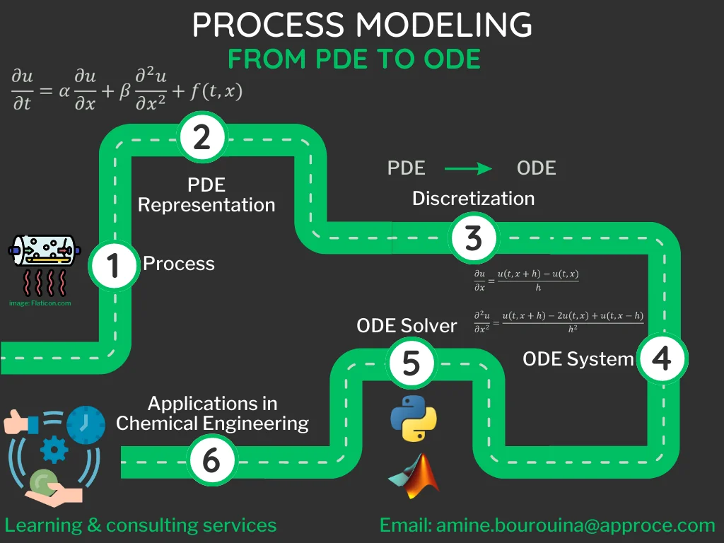
Finite differences

For a one-dimensional grid with spacing $\Delta x$,

For the heat equation, a forward-Euler scheme gives

where

In one spatial dimension, this explicit scheme is stable only when

Numerical stability is therefore part of the model implementation. A solver can produce numbers and still be mathematically invalid.

Finite elements

Finite-element methods start from a weak formulation. For a Poisson equation

multiply by test function $v$ and integrate:

after integration by parts and suitable boundary conditions. The solution is approximated in a finite-dimensional basis. This is especially useful on irregular geometries. The method is not simply “breaking the domain into pieces”; the weak formulation is what makes finite elements mathematically distinctive.

Data assimilation

Data assimilation combines a dynamical model with sequential observations. A state-space representation is

Here $M$ may contain a discretized PDE solver. Kalman filters, ensemble Kalman filters, and variational assimilation methods estimate latent states while respecting both model dynamics and observations. Weather prediction is a major example.

Surrogate models

If a PDE solver costs minutes or hours per evaluation, inference requiring thousands of evaluations becomes expensive. A surrogate approximates

with a cheaper model

Options include:

• Gaussian processes;
• polynomial chaos;
• reduced-order bases;
• neural operators;
• conventional neural networks.

The surrogate error must be propagated into the final inference when it is not negligible.

Physics-informed neural networks

A PINN represents a solution $u_\phi(x,t)$ with a neural network and penalizes violations of the PDE. For

a residual is

A training loss might combine

This is elegant. It is not automatically superior to finite differences or finite elements. PINNs can struggle with stiffness, multiscale structure, sharp fronts, optimization pathology, and badly balanced loss terms. The benchmark should always include a conventional numerical solver when one is available.

Neural operators

A standard neural network learns a finite-dimensional function. A neural operator aims to learn a map between functions, for example

where $a$ is a PDE coefficient field and $u$ the corresponding solution field. This can be useful when many related PDE solves are required. Again, the key use case is amortization:

PDEs versus stochastic differential equations

An SDE such as

is not a PDE. But the probability density or expected-value function associated with an SDE often satisfies a PDE such as the Fokker-Planck or backward Kolmogorov equation. In finance, the Black-Scholes PDE can be derived from a stochastic asset model under assumptions. The connection is mathematical, not terminological equivalence.

Image processing

Diffusion PDEs have long been used in image processing. Linear diffusion smooths noise but also blurs edges. Anisotropic diffusion modifies the diffusion coefficient to reduce smoothing across strong gradients. This is an example of model structure encoding a desired property. It predates modern deep learning and remains conceptually useful.

What data scientists should learn

The most transferable concepts are not a catalogue of PDE names. They are:

1. state versus observation;
2. forward versus inverse problem;
3. well-posedness and identifiability;
4. discretization error;
5. stability and convergence;
6. regularization;
7. uncertainty propagation.

These ideas recur in statistical learning even when no PDE appears explicitly.

Conclusion

PDEs matter to data science when data are partial observations of a structured dynamical system. The central chain is

Machine learning becomes useful when it accelerates, regularizes, or augments this chain. It should not replace the mathematical structure without evidence that the replacement works.

References

• Evans, L. C. (2010). Partial Differential Equations (2nd ed.). American Mathematical Society.
• LeVeque, R. J. (2007). Finite Difference Methods for Ordinary and Partial Differential Equations. SIAM.
• Stuart, A. M. (2010). Inverse problems: A Bayesian perspective. Acta Numerica, 19, 451–559.
• Raissi, M., Perdikaris, P., & Karniadakis, G. E. (2019). Physics-informed neural networks. Journal of Computational Physics, 378, 686–707.