Mastering Bayesian Statistics: An In-Depth Guide to MCMC

Complex Probabilities with Markov Chain Monte Carlo

21 minute read

Example Image

Markov Chain Monte Carlo

Introduction to Bayesian Statistics and MCMC

Brief Overview of Bayesian Statistics

Bayesian statistics presents a framework for incorporating prior knowledge and evidence into the statistical analysis process. Unlike frequentist statistics, which interprets probability as the long-run frequency of events, Bayesian statistics views probability as a measure of believability or certainty in an event. This approach fundamentally hinges on Bayes’ theorem, which updates the probability estimate for a hypothesis as more evidence or information becomes available.

In Bayesian analysis, we use the prior distribution to express our initial beliefs about a parameter before observing the data. Once data is observed, the prior is updated using the likelihood function, which measures how probable the observed data is under different parameter values, leading to the posterior distribution. The posterior distribution then becomes a new, refined view of the parameter’s probability, incorporating both our prior beliefs and the observed data.

The Significance of MCMC in Bayesian Analysis

Markov Chain Monte Carlo (MCMC) methods are crucial in Bayesian statistics, primarily because they allow us to approximate complex posterior distributions that are often analytically intractable. MCMC methods, like Metropolis-Hastings and Gibbs sampling, generate samples from the posterior distribution, which can then be used to estimate various statistical properties.

One of the primary reasons MCMC is so significant in Bayesian analysis is its flexibility and generality. MCMC methods can be applied to a wide range of problems, regardless of the complexity of the model or the prior distributions involved. They provide a powerful tool for performing Bayesian inference, especially in high-dimensional spaces where traditional methods falter.

Challenges in Computing Bayesian Probabilities

Despite its powerful capabilities, MCMC is not without its challenges. One of the key difficulties lies in ensuring the convergence of the Markov Chain to the true posterior distribution. If not run for a sufficient amount of time, or if improperly configured, MCMC methods can yield misleading results.

Another challenge is the computational cost, especially for complex models or large datasets. MCMC algorithms can be computationally intensive, requiring significant time and resources to produce accurate estimates. This is particularly problematic in real-time analytics or scenarios where rapid decision-making is crucial.

Lastly, choosing appropriate priors and constructing likelihood functions that accurately reflect the data can be non-trivial tasks. Mis-specification of these components can lead to biased or incorrect inferences, undermining the reliability of Bayesian analysis.

Despite these challenges, the power and flexibility of MCMC methods continue to make them a cornerstone in the field of Bayesian statistics, providing a pathway to tackle complex probabilistic models in a variety of scientific and analytical domains.

Understanding Bayes’ Theorem

Explanation of Bayes’ Theorem Components

Bayes’ Theorem is a fundamental concept in probability theory and statistics, forming the backbone of Bayesian analysis. It is expressed as:

Bayes’ Formula is expressed as: \(P(\theta \mid X) = \frac{P(X \mid \theta) \cdot P(\theta)}{P(X)}\)

Where:

\(P(\theta \mid X)\) is the posterior probability. It represents the probability of the hypothesis \(\theta\) given the observed data \(X\).
\(P(X \mid \theta)\) is the likelihood. It indicates the probability of observing the data \(X\) given that the hypothesis \(\theta\) is true.
\(P(\theta)\) is the prior probability. This is our initial belief about the hypothesis before observing the data.
\(P(X)\), the evidence, is the probability of observing the data under all possible hypotheses. It acts as a normalizing constant to ensure that the posterior probabilities sum up to one.

The Role of Priors, Likelihood, and Evidence

Priors: The prior \(P(\theta)\) encapsulates existing knowledge or beliefs about the hypothesis before considering the current data. Priors can be subjective, based on expert opinion, or objective, derived from historical data or other sources. The choice of prior can significantly influence the results, especially with limited data.
Likelihood: The likelihood \(P(X \mid \theta)\) measures how probable the observed data is under various hypotheses. It plays a crucial role in updating the prior beliefs in light of new data. In statistical modeling, the likelihood often embodies the model or the assumed data-generating process.
Evidence: Although \(P(X)\) is often challenging to calculate directly, it ensures that the posterior probabilities are properly scaled. In practice, this term is usually handled by normalization or algorithms like MCMC, which circumvent the need to calculate it explicitly.

Real-World Application Examples

Medical Diagnosis: Bayesian methods are used in diagnostics to update the probability of a disease as more patient information becomes available. For instance, the prior probability of a disease could be based on prevalence rates, which is then updated with likelihoods derived from test results to provide a more accurate diagnosis.
Machine Learning: In machine learning, Bayesian methods are used for regularization and avoiding overfitting. Priors can encode preferences or constraints in the model, and the updating process with data helps in making robust predictions.
Finance and Risk Management: Bayesian statistics are employed to model market uncertainties. Prior market beliefs are updated with incoming financial data to assess risks and make investment decisions.
Environmental Science: In climate modeling, priors on climate sensitivity are updated with observational data to predict future climate changes more accurately.

These examples demonstrate the versatility of Bayesian methods across various fields, showing how initial assumptions can be systematically revised with new evidence, leading to more informed decisions and predictions.

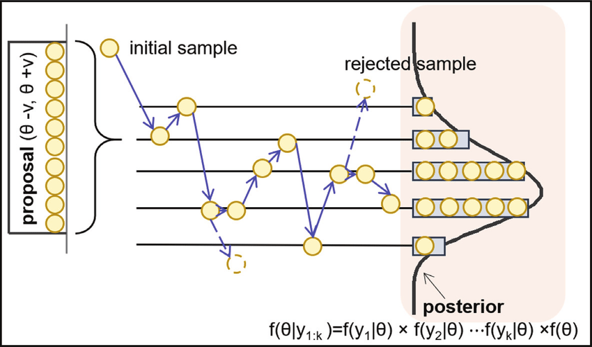
The Mechanics of MCMC

Introduction to Markov Chains

A Markov Chain is a mathematical system that transitions from one state to another within a finite or countable number of possible states. It’s defined by its property of being “memoryless” — the next state depends only on the current state and not on the sequence of events that preceded it. This property is known as the Markov property.

In the context of MCMC, Markov Chains are used to model the random variables of interest. The chain moves stepwise through a series of states (which represent possible values of these variables) in such a way that the long-term proportion of time spent in each state converges to the probability of that state according to the target distribution (usually the posterior distribution in Bayesian analysis).

How MCMC Navigates Probability Distributions

MCMC methods generate samples from a probability distribution by constructing a Markov Chain whose equilibrium distribution matches the target distribution. The basic idea is to create a random walk using a proposal distribution and a set of rules for accepting or rejecting proposed moves. This process ensures that the chain will eventually reach and spend time in regions of the probability space in proportion to their density under the target distribution.

The most common MCMC method, the Metropolis-Hastings algorithm, involves generating a sequence of sample values in such a way that, even though the sequence itself may be dependent, the distribution of the sequence converges to the desired distribution. This is achieved through a ‘proposal’ mechanism for suggesting new samples and an ‘acceptance’ criterion to decide whether these proposals are accepted or rejected, based on how likely they are under the target distribution.

Comparison with Traditional Methods

MCMC methods differ significantly from traditional statistical methods, which might rely on direct sampling or analytical solutions. Where traditional methods struggle - particularly in high-dimensional spaces or with complex, non-standard probability distributions - MCMC methods thrive.

Sampling Complexity: Traditional direct sampling methods require samples to be independently drawn from the target distribution, which is often not feasible for complex distributions. MCMC, however, cleverly constructs a dependent sequence of samples that still accurately represents the target distribution.
Analytical Solutions: Many statistical problems, especially in Bayesian statistics, do not have closed-form solutions. MCMC methods bypass the need for an analytical solution by providing a way to estimate properties of the distribution through simulation.
Flexibility: MCMC methods are highly adaptable to various types of data and models. They can be used with a wide range of priors and likelihoods in Bayesian analysis, something that traditional methods may not accommodate easily.

In summary, MCMC methods extend the reach of statistical analysis into areas where traditional methods are not practical or possible, offering a powerful tool for inference in complex probabilistic models.

Key MCMC Algorithms

Overview of Metropolis-Hastings

The Metropolis-Hastings algorithm is a cornerstone of MCMC methods, widely used for its simplicity and versatility. It’s an extension of the Metropolis algorithm and allows for a broader range of proposal distributions. The algorithm follows these steps:

Start with an Initial Guess: Begin with an initial value for the parameters of interest.
Generate a Proposal: At each step, propose a new set of parameter values. This proposal is generated from a distribution centered around the current values.
Calculate Acceptance Ratio: Compute the ratio of the posterior probabilities of the new and current parameters. This ratio is adjusted by the ratio of the proposal densities if the proposal distribution is asymmetric.
Accept or Reject: Compare the acceptance ratio to a random number drawn from a uniform distribution. If the ratio is greater, accept the new values; otherwise, keep the current ones.
Repeat: Repeat the process for a large number of iterations. The Metropolis-Hastings algorithm is particularly effective in exploring the parameter space and approximating complex posterior distributions.

Introduction to Gibbs Sampling

Gibbs Sampling is a special case of the Metropolis-Hastings algorithm and is used when the joint distribution is difficult to sample from, but the conditional distributions are tractable. It’s particularly useful in high-dimensional problems. The steps are:

Initial Start: Choose initial values for all the parameters.
Sequential Updating: Update each parameter in turn, holding all others fixed. Draw the new value for the current parameter from its conditional distribution given the current values of all other parameters.
Iterate: Cycle through all parameters repeatedly, updating them sequentially.
Convergence: After many iterations, the distribution of values converges to the joint posterior distribution of the parameters. Gibbs Sampling is efficient when the conditional distributions are easier to sample from than the joint distribution, a common scenario in complex Bayesian models.

Discussion on other variants (e.g., Slice Sampling)

There are several other variants of MCMC, each with unique advantages in specific scenarios:

Slice Sampling: This method addresses the difficulty of choosing a good proposal distribution in Metropolis-Hastings. It involves ‘slicing’ the distribution at a random height and then sampling uniformly from the horizontal ‘slice’ defined by this height. It’s particularly useful for reducing correlation between successive samples.
Hamiltonian Monte Carlo (HMC): This variant uses concepts from physics to inform the proposal mechanism. It’s especially effective in high-dimensional spaces, reducing the random walk behavior and correlated samples often seen in simpler MCMC methods.
Reversible Jump MCMC: This advanced method allows for variable-dimensional parameter spaces, facilitating model comparison and variable selection within a Bayesian framework.

Each of these algorithms has specific applications where it excels, and the choice of algorithm often depends on the problem at hand, the complexity of the model, and the desired efficiency and accuracy of the sampling process.

Implementing MCMC in Python

Setting up a Python Environment for Statistical Computing

To implement MCMC in Python, a proper environment setup is essential. This typically includes installing Python and necessary libraries. The key libraries for MCMC and statistical computing include:

numpy: For numerical operations.
scipy: Provides additional functionality and statistical methods.
matplotlib or seaborn: For data visualization.
pandas: For data manipulation and analysis.
MCMC-specific libraries like pymc3 or emcee. You can set up this environment using Python’s package manager pip or a package management system like Anaconda, which simplifies managing dependencies and libraries.

Coding Example with Explanations

Here’s a simple example of implementing the Metropolis-Hastings algorithm in Python:

import numpy as np
import scipy.stats as stats
import matplotlib.pyplot as plt

# Define the likelihood and the prior
def likelihood(theta, data):
    return stats.norm(theta, 1).pdf(data).prod()

def prior(theta):
    return stats.norm(0, 1).pdf(theta)

# Metropolis-Hastings algorithm
def metropolis_hastings(likelihood, prior, data, initial_theta, iterations, proposal_width):
    theta = initial_theta
    accepted = []
    
    for i in range(iterations):
        theta_proposal = theta + proposal_width * np.random.randn()
        
        # Compute the acceptance probability
        ratio = likelihood(theta_proposal, data) * prior(theta_proposal) / \
                (likelihood(theta, data) * prior(theta))
        acceptance_probability = min(1, ratio)
        
        # Accept or reject the proposal
        if np.random.rand() < acceptance_probability:
            theta = theta_proposal
            accepted.append(theta_proposal)
    
    return np.array(accepted)

# Generate some data
data = np.random.randn(20)

# Run the MCMC sampler
accepted_samples = metropolis_hastings(likelihood, prior, data, initial_theta=0, iterations=10000, proposal_width=0.5)

# Plotting
plt.hist(accepted_samples, bins=30, density=True)
plt.xlabel("Theta")
plt.ylabel("Frequency")
plt.title("Posterior Distribution of Theta")
plt.show()

In this example, we define a simple Gaussian likelihood and prior. The metropolis_hastings function takes these, along with data and initial parameter values, and runs the MCMC algorithm for a specified number of iterations.

Analysis of MCMC Output and Convergence

Visual Inspection: Plotting the histogram of the accepted samples gives us an insight into the posterior distribution. We expect it to approximate the true distribution after a sufficient number of iterations.
Convergence Diagnostics: There are several methods to check for convergence:
- Trace plots: Plot the sequence of accepted values against iteration number. Convergence is indicated if the plot reaches a stationary state.
- Autocorrelation: Analyze the autocorrelation of the accepted samples. Lower autocorrelation at increasing lags suggests good mixing of the chain.
- Gelman-Rubin Diagnostic: Compare multiple chains with different starting values. Convergence is indicated by the chains mixing well, assessed quantitatively by the diagnostic value (close to 1 suggests convergence).
Burn-in and Thinning: The initial samples (‘burn-in’) may not be representative of the target distribution and are often discarded. Additionally, ‘thinning’ (keeping every nth sample) can be used to reduce autocorrelation in the sample set.

Proper analysis of MCMC output is crucial for making reliable statistical inferences. It ensures that the samples used represent the posterior distribution accurately, thus making the conclusions drawn from the analysis more robust.

Advanced Applications of MCMC

MCMC methods are not just limited to simple statistical models; they have profound applications in more complex scenarios. These include hierarchical models, mixture models, and change point detection, each presenting unique challenges that MCMC is particularly well-suited to address.

MCMC in Complex Models

Hierarchical Models: Hierarchical or multi-level models involve parameters that are themselves random variables with their own distributions. These models are common in data with natural groupings, allowing for shared information between groups. MCMC is ideal for these models as it can efficiently handle the dependencies and varying levels of uncertainty within the hierarchical structure.
Mixture Models: Mixture models are used when data is thought to be generated from several different processes or distributions, but it’s unclear which observation comes from which process. MCMC helps in estimating the parameters of the individual distributions and the probability that each observation belongs to each distribution.
Change Point Detection: In time series data, change point detection identifies points in time where the statistical properties of a sequence of observations change significantly. MCMC can be used to estimate the posterior distribution of the number and locations of these change points, as well as the parameters of the different segments of the data.

Case Studies and Industry Applications

Ecology and Environmental Science: In ecology, hierarchical models are used to understand complex ecological dynamics. MCMC has been employed to model animal population dynamics, where different levels of the hierarchy might represent individual animal behavior and population-level dynamics.
Finance and Economics: MCMC methods are used in econometrics for parameter estimation in complex models of economic behavior. In finance, they assist in risk assessment models and in identifying regime changes in financial time series data.
Genetics and Bioinformatics: In genetics, MCMC is used in models that estimate the genetic structure of populations or the evolutionary relationships between different species. It’s especially useful in Bayesian phylogenetics and genome-wide association studies.
Medical Research: Hierarchical models via MCMC are applied in clinical trials and epidemiological studies. They help in understanding the effects of treatments or interventions across different groups and subpopulations.
Machine Learning: In the realm of machine learning, MCMC methods are used in Bayesian neural networks and for optimizing hyperparameters in complex models.
Quality Control and Manufacturing: MCMC aids in detecting changes in manufacturing processes, ensuring quality control by identifying points where the process deviates from the norm.

These advanced applications demonstrate the versatility of MCMC methods. They allow for robust and nuanced analysis across various disciplines, handling complexities and uncertainties that are otherwise challenging to address with more traditional statistical approaches.

MCMC with Python Libraries

Python, being a versatile programming language, offers powerful libraries specifically designed for implementing Markov Chain Monte Carlo (MCMC) methods. Two of the most prominent libraries in this domain are PyMC and PyStan. Both provide robust tools for performing Bayesian inference but have distinct characteristics and features.

Leveraging PyMC and PyStan for MCMC

PyMC: PyMC3 (the latest version) is a Python library that specializes in probabilistic programming. It allows users to write down models using an intuitive syntax to describe the statistical model. PyMC3 includes a comprehensive set of pre-defined statistical distributions and model fitting algorithms, including MCMC. It leverages Theano for automatic differentiation and GPU support, which can significantly accelerate computation.

Key Features:
- Intuitive model specification syntax.
- Powerful sampling algorithms like the No-U-Turn Sampler (NUTS), a variant of Hamiltonian Monte Carlo (HMC).
- Extensive variety of built-in probability distributions.
- Advanced features for model diagnostics and comparison.

import pymc3 as pm
import numpy as np

# Example: Simple linear regression model
X = np.random.randn(100)
y = 3 * X + np.random.randn(100)

with pm.Model() as model:
    # Defining the model
    intercept = pm.Normal('Intercept', mu=0, sigma=10)
    slope = pm.Normal('Slope', mu=0, sigma=10)
    sigma = pm.HalfNormal('sigma', sigma=1)
    
    # Expected value
    mu = intercept + slope * X
    
    # Likelihood
    Y_obs = pm.Normal('Y_obs', mu=mu, sigma=sigma, observed=y)
    
    # Inference
    trace = pm.sample(2000)

PyStan: PyStan is the Python interface to Stan, a state-of-the-art platform for statistical modeling and high-performance statistical computation. Stan uses an expressive programming language for specifying complex statistical models and implements advanced MCMC algorithms like HMC.

Key Features:
- Provides a powerful and flexible modeling language.
- Efficient samplers that handle high-dimensional parameter spaces well.
- Integrates well with the larger Stan ecosystem, allowing users to access advanced modeling techniques.
- Good for high-dimensional and complex models.

import pystan
import pandas as pd

# Example: Simple linear regression model
data = {'N': 100, 'x': X, 'y': y}
code = '''
data {
    int<lower=0> N;
    vector[N] x;
    vector[N] y;
}
parameters {
    real alpha;
    real beta;
    real<lower=0> sigma;
}
model {
    y ~ normal(alpha + beta * x, sigma);
}
'''

# Model fitting
sm = pystan.StanModel(model_code=code)
fit = sm.sampling(data=data, iter=2000, chains=4)

Comparative Analysis of Library Features

Ease of Use: PyMC3 generally has a more Pythonic, user-friendly interface, making it more accessible for beginners. PyStan, while powerful, has a steeper learning curve due to its distinct modeling language.
Performance: PyStan is known for its efficient sampling algorithms and can be faster in some complex models, especially those with high-dimensional parameter spaces. PyMC3, with Theano’s optimization, also offers efficient and fast computation but may lag behind in very complex models.
Modeling Flexibility: Both libraries provide extensive support for a wide range of statistical distributions and complex models. PyStan’s modeling language is more expressive but can be more verbose.
Community and Support: PyMC3 has a large and active community, offering extensive resources, tutorials, and support. PyStan benefits from being part of the broader Stan community, which is well-established and has a wealth of expertise in statistical modeling.

In summary, the choice between PyMC3 and PyStan often depends on the specific requirements of the project, the user’s familiarity with Python and statistical modeling languages, and the complexity of the models being developed. Both libraries are powerful tools in the arsenal of a data scientist or statistician working with Bayesian methods.

Challenges and Best Practices in MCMC

Implementing Markov Chain Monte Carlo (MCMC) methods can be challenging, and there are common pitfalls that practitioners often encounter. However, adhering to best practices can significantly enhance the accuracy and efficiency of MCMC simulations.

Common Pitfalls in MCMC Implementations

Convergence Issues: One of the most common issues with MCMC is non-convergence, where the Markov chain fails to adequately explore the entire parameter space, leading to biased estimates. This often occurs in complex models or when the proposal distribution is poorly chosen.
Autocorrelation: High autocorrelation among samples can lead to inefficient sampling, where a large number of iterations are required to obtain a relatively small amount of independent information about the posterior distribution.
Poor Mixing: Poor mixing occurs when the Markov chain gets stuck in a particular region of the parameter space for a prolonged period. This is often a sign that the parameter space is not being explored efficiently.
Improper Scaling: In high-dimensional models, improper scaling of the proposal distribution can lead to either an excessive number of rejections (if too large) or an inefficient random walk exploration (if too small).
Model Mis-specification: Incorrectly specified models or priors that don’t reflect prior knowledge or data characteristics can lead to incorrect inferences.

Tips for Ensuring Accurate and Efficient Simulations

Monitor Convergence: Utilize diagnostic tools to assess convergence. This includes visual methods like trace plots, as well as quantitative measures like the Gelman-Rubin statistic. Run multiple chains with different starting points to ensure that they converge to the same distribution.
Address Autocorrelation: Use thinning (i.e., selecting every nth sample) to reduce autocorrelation, though this is not a substitute for running a sufficiently long chain. Consider using advanced MCMC algorithms that are designed to reduce autocorrelation, such as Hamiltonian Monte Carlo (HMC).
Tune the Proposal Distribution: In algorithms like Metropolis-Hastings, carefully tune the proposal distribution. Adaptive MCMC methods, which adjust the proposal distribution on the fly, can be particularly useful.
Ensure Proper Scaling: For high-dimensional problems, ensure that the scaling of the proposal distribution is appropriate. This may involve tuning hyperparameters or using algorithms that adaptively scale proposals.
Validate the Model: Perform model checking and validation to ensure that the model adequately fits the data. This can involve posterior predictive checks or comparing model outputs to known or simulated data.
Use Informative Priors: When possible, use informative priors to guide the sampling process, especially in models with weak or noisy data.
Leverage Parallel Computing: Utilize parallel computing resources to run multiple chains or for computationally intensive models. Many MCMC libraries support parallelization.
Expertise and Experience: Given the complexity and subtleties of MCMC, input from experienced statisticians can be invaluable, especially when dealing with complex models or interpreting results.

By being aware of these challenges and employing best practices, practitioners can greatly improve the reliability and efficiency of MCMC simulations, leading to more robust and trustworthy conclusions in their statistical analyses.

Conclusion

Recap of MCMC’s Importance in Bayesian Analysis

Throughout this exploration of Markov Chain Monte Carlo (MCMC) methods, their integral role in Bayesian analysis has been consistently evident. MCMC provides a robust set of tools for approximating complex posterior distributions, particularly in scenarios where traditional analytical approaches fall short. Its flexibility and adaptability in handling a wide range of models, from simple to highly intricate ones, make MCMC an indispensable method in modern statistical analysis and data science.

Key points to remember about MCMC in Bayesian analysis include:

Handling Complex Models: MCMC excels in managing high-dimensional parameter spaces and intricate probability distributions, making it possible to glean insights from complex Bayesian models.
Incorporating Prior Knowledge: It allows for the seamless integration of prior information, updating beliefs in light of new data to generate posterior distributions.
Versatility and Wide Application: MCMC’s application spans various fields, from genetics and ecology to finance and machine learning, demonstrating its versatility and broad utility.

Future Directions and Evolving Trends in MCMC Research

As the field of statistics and data science continues to evolve, so too will the methodologies and applications of MCMC. Key areas of future development and research include:

Algorithmic Improvements: Ongoing research is focused on developing more efficient and faster-converging MCMC algorithms. This includes enhancing existing algorithms and inventing new ones to tackle increasingly complex models.
Automated Tuning Processes: Efforts are being made to automate the tuning of MCMC parameters, reducing the need for manual intervention and making MCMC more accessible to a broader user base.
Integration with Machine Learning: There is a growing intersection between Bayesian methods, including MCMC, and machine learning. This includes using MCMC in deep learning for Bayesian neural networks and in reinforcement learning for decision-making under uncertainty.
Scalability and Big Data: As data continues to grow in size and complexity, scaling MCMC algorithms to handle big data efficiently is a significant research focus.
Interdisciplinary Collaboration: Increased collaboration between statisticians, computer scientists, domain experts, and practitioners is expected to lead to the development of innovative MCMC applications and improvements.
User-Friendly Software Development: The development of more intuitive and user-friendly MCMC software, along with educational resources, will likely continue, making these powerful methods more accessible to non-specialists.

In conclusion, MCMC methods are poised to remain at the forefront of Bayesian analysis and probabilistic modeling. Their ability to address the challenges of complex data analysis ensures their ongoing relevance and application in a multitude of disciplines, continually expanding the frontiers of knowledge and data-driven decision-making.