Distinguishing Ergodic Regimes from Processes

Abstract

Ergodicity, a foundational concept across disciplines such as physics, chemistry, natural sciences, economics, and machine learning, often suffers from a widespread misconception. Traditionally, ergodicity has been attributed to processes themselves, suggesting that a process can be inherently ergodic. This perspective, however, overlooks the nuanced understanding that ergodicity is not a fixed property but a regime or condition that emerges within the temporal evolution of a process. The distinction is critical for accurate analysis and interpretation in theoretical and applied research. This paper aims to elucidate the misconception by advocating for a shift in perspective: from identifying “ergodic processes” to recognizing “ergodic regimes” based on observables and their evolution over time. Through a detailed examination of ergodicity measures, mathematical formulations, and a case study on Bernoulli Trials, we underscore the importance of this paradigm shift for a deeper understanding of ergodic behavior in complex systems.

Introduction

Ergodicity is a cornerstone concept that intersects multiple fields of science, including physics, chemistry, the natural sciences, and more recently, economics and machine learning. Its significance lies in understanding how systems evolve over time and the implications of this evolution for predicting future states. Despite its widespread application, the definition and interpretation of ergodicity vary, leading to confusion and misconceptions, particularly regarding its application to processes and regimes.

The concept of ergodicity was originally introduced to reconcile the macroscopic observations of thermodynamic systems with their microscopic statistical behaviors. In its most general sense, ergodicity describes a system’s property where its time average is equal to its ensemble average. However, the journey from this broad description to practical application is fraught with complexity, especially when distinguishing between Birkhoff’s statistical definition and Boltzmann’s physical approach. This paper adheres to Birkhoff’s perspective, which emphasizes the statistical nature of ergodicity, framing it as a property that emerges from the long-term behavior of a system rather than its instantaneous state.

One prevalent misconception is the characterization of processes as inherently ergodic. This view simplifies ergodicity to a binary attribute of a process, ignoring the intricate dependencies on initial conditions, the nature of observables, and the temporal window over which observations are made. Such a simplification not only misrepresents the theory but also undermines the practical analysis and interpretation of systems where ergodicity is a relevant concern.

Understanding ergodicity as a regime rather than an inherent process characteristic necessitates a paradigm shift. It requires recognizing that ergodic behavior is contingent on specific conditions and parameters, including the choice of observable and the time scale of observation. This nuanced view opens the door to a more accurate and meaningful analysis of systems, enabling researchers to identify when and how ergodicity manifests in the evolution of a process.

In this introduction, we explore the roots of the ergodicity concept, clarify the statistical underpinnings as posited by Birkhoff, and address the critical misconception surrounding ergodic processes. We argue for the importance of identifying ergodic regimes within the temporal evolution of processes, a perspective that not only aligns with theoretical foundations but also enhances the practical understanding and application of ergodic principles across diverse scientific disciplines.

Ergodicity in Theory and Practice

Definitions and Background

Ergodicity is a fundamental concept with far-reaching applications across a multitude of scientific disciplines. At its core, ergodicity provides a framework for understanding the dynamics of systems over time, bridging the microscopic and macroscopic worlds, especially in the context of statistical mechanics, thermodynamics, and beyond. This section delves into the multifaceted nature of ergodicity, exploring its significance in various fields and elucidating the distinctions between two foundational approaches to its definition: those of Birkhoff and Boltzmann.

Ergodicity Across Disciplines:

• Physics: In physics, ergodicity is instrumental in explaining the thermodynamic behavior of systems at equilibrium. It underpins the statistical mechanics framework, allowing for the prediction of macroscopic properties based on the behavior of microscopic constituents.
• Chemistry: Chemical physics and molecular dynamics utilize the concept of ergodicity to describe the time evolution of molecular systems, aiding in the understanding of reaction dynamics, equilibration, and transport phenomena.
• Natural Sciences: Ergodicity finds application in the study of ecological and evolutionary dynamics, providing insights into population behaviors and environmental interactions over time.
• Economics: The adoption of ergodicity in economics facilitates modeling under uncertainty, addressing how economic agents make decisions over time in the face of fluctuating markets and information.
• Machine Learning: In the realm of machine learning, ergodicity is relevant in stochastic optimization and the analysis of algorithms, particularly in understanding the convergence properties of Markov chain Monte Carlo methods.

Birkhoff vs. Boltzmann on Ergodicity:

The concept of ergodicity has evolved, with significant contributions from George David Birkhoff and Ludwig Boltzmann, each offering a perspective that highlights different aspects of the theory:

• Boltzmann’s Physical Approach: Boltzmann’s interpretation, rooted in the physical sciences, emphasizes the idea that a system, given enough time, will pass through every conceivable state compatible with its energy. This approach is closely tied to the physical intuition of systems exploring their entire phase space, a concept foundational to classical thermodynamics and statistical mechanics.
• Birkhoff’s Statistical Definition: Birkhoff shifted the focus towards a more mathematical and statistical framework. His definition of ergodicity hinges on the equivalence of time averages and ensemble averages for a system. Specifically, Birkhoff’s ergodic theorem formalizes the conditions under which the long-term average of a function over the phase space of a system is equal to the average over its entire accessible states, providing a rigorous statistical foundation for the concept.

The distinction between Birkhoff’s and Boltzmann’s definitions underscores a pivotal shift from a physically intuitive to a statistically rigorous understanding of ergodicity. Birkhoff’s approach, with its emphasis on statistical properties and long-term averages, offers a more generalizable framework that extends beyond the physical sciences, accommodating the complexities and nuances of systems observed in chemistry, economics, and beyond. This evolution in the conceptualization of ergodicity not only broadens its applicability but also deepens our understanding of dynamic systems across disciplines.

In summary, ergodicity encapsulates a critical principle for the analysis of systems in equilibrium and non-equilibrium states alike. By distinguishing between the physical intuition of Boltzmann and the statistical rigor of Birkhoff, we gain a comprehensive understanding of how ergodicity functions across theoretical and applied contexts, paving the way for its nuanced application in addressing complex phenomena in science and beyond.

Misconception of Ergodic Process

The concept of ergodicity, while widely recognized across various scientific disciplines, is often accompanied by a fundamental misconception regarding its nature and application. This misunderstanding centers on the notion of ergodic processes—a term that suggests a static attribute of a process, implying that a process is either ergodic or non-ergodic in its entirety. This section aims to clarify this misconception and introduce a more nuanced understanding of ergodic regimes within the temporal evolution of processes.

Common Misunderstanding**

The prevalent misunderstanding arises from a simplistic interpretation of ergodicity, where it is viewed as an inherent property of a system or process. According to this perspective, if a process is labeled “ergodic,” it is expected to exhibit ergodic behavior under all conditions and across all time scales. This interpretation overlooks the critical role of observables and the specific temporal and spatial scales at which the system is analyzed. Ergodicity, in its essence, is not a blanket characteristic that applies universally but a condition that emerges under certain constraints and parameters.

Ergodic Regimes vs. Ergodic Processes

To address the misconception, it is essential to differentiate between the concepts of ergodic processes and ergodic regimes. An ergodic regime refers to a specific condition or window in the temporal evolution of a system where the ergodic property—namely, the equivalence of time averages and ensemble averages for a given observable—holds true. This regime is not a permanent attribute but a dynamic state that can depend on multiple factors, including the system’s initial conditions, external influences, and the nature of the observables considered.

• Role of Observables: The ergodicity of a system is intimately linked to the observables under study. Different observables derived from the same process can lead to varying conclusions about the system’s ergodicity. This highlights the importance of clearly defining the observables and understanding their behavior over time.
• Temporal and Spatial Scales: The detection of ergodic regimes is also influenced by the temporal and spatial scales at which the system is observed. A process may appear non-ergodic over short time scales but exhibit ergodic behavior when observed over sufficiently long periods. Similarly, the spatial scale and granularity of observation can affect the assessment of ergodicity.

Implications of Recognizing Ergodic Regimes

Understanding ergodicity as a regime rather than an inherent property of processes has profound implications for theoretical and empirical research. It allows for a more flexible and accurate description of system dynamics, accommodating the complex behavior of real-world systems that may transition between ergodic and non-ergodic states. This perspective encourages researchers to focus on the conditions under which ergodicity is observed, facilitating a deeper understanding of the mechanisms driving system behavior.

In conclusion, the transition from viewing processes as inherently ergodic to recognizing the existence of ergodic regimes enriches our understanding of dynamic systems. It underscores the importance of context, observables, and scales in the analysis of ergodicity, paving the way for more nuanced and accurate scientific inquiries into the nature of complex systems.

Identifying Ergodic Regimes

Key Components

To accurately identify and analyze ergodic regimes within a process, it is crucial to understand several foundational concepts that underpin the theory of ergodicity. These include the ensemble, observable, process, measure, and threshold. Each plays a pivotal role in determining whether a specific regime can be considered ergodic. This understanding is essential for the precise application of ergodic theory across various scientific disciplines.

Ensemble: An ensemble represents a collection or set of all possible states or configurations that a system can assume. In the context of statistical mechanics, for example, an ensemble might encompass all the microstates consistent with a given energy level. The concept of an ensemble allows for the statistical treatment of systems by considering all possible outcomes or configurations simultaneously, providing a foundation for ensemble averages.

Observable: An observable is a quantifiable property or characteristic of a system that can be measured or computed. In physical sciences, observables could include properties like energy, momentum, or position. In economics, observables might involve indicators such as prices, interest rates, or consumption levels. The choice of observable is critical in ergodic theory, as it directly influences the assessment of whether a system’s time averages and ensemble averages align.

Process: A process refers to the evolution of a system over time, governed by a set of underlying dynamics. Processes can be deterministic, where future states of the system are precisely determined by its current state, or stochastic, where evolution involves randomness or probability. The nature of the process, including its sensitivity to initial conditions or external perturbations, is a key factor in determining the system’s ergodic behavior.

Measure and Threshold: The measure of ergodicity is a quantitative criterion used to assess the equivalence between time averages and ensemble averages for a given observable. This measure often involves calculating the difference or ratio between these two averages and comparing it to a predefined threshold. The threshold determines the degree of similarity required for a system to be considered ergodic. A small measure relative to the threshold suggests that the system is in an ergodic regime for the observable in question.

Different Observables and Ergodic Regimes: The ergodicity of a system is not a monolithic property but is highly dependent on the specific observable under consideration. Different observables derived from the same process can lead to different conclusions about ergodicity. For instance, one observable might exhibit ergodic behavior, with its time average converging to the ensemble average, while another observable does not. This discrepancy arises because different observables can be sensitive to different aspects of the system’s dynamics or interact with the underlying process in unique ways.

The identification of ergodic regimes, therefore, requires a careful and nuanced approach that takes into account the specific observables, the nature of the process, and the criteria for measuring ergodicity. By systematically analyzing these components, researchers can more accurately determine when and how ergodicity manifests in complex systems, facilitating a deeper understanding of their long-term behavior and statistical properties.

In summary, the task of identifying ergodic regimes hinges on a detailed examination of key concepts such as the ensemble, observable, process, measure, and threshold. Recognizing how different observables can lead to varying ergodic outcomes underscores the importance of a tailored approach to the analysis of ergodicity, accommodating the intricacies and diversity of dynamic systems across scientific fields.

Mathematical Formulation

To rigorously identify and analyze ergodic regimes, it’s essential to frame the discussion within the context of mathematical formulation. Processes, whether observed in the natural world or conceptualized in theoretical models, can often be described as dynamical systems. These systems are characterized by rules that dictate how the state of the system evolves over time. The mathematical study of these evolutions provides a deep understanding of ergodic regimes, differentiating between stochastic and deterministic models and elucidating what constitutes a regime from a mathematical standpoint.

Processes as Dynamical Systems

Deterministic Models: In deterministic dynamical systems, the future state of the system is completely determined by its current state, without any randomness in the evolution. The equations governing such systems are typically differential or difference equations, where time plays a crucial role. Deterministic models are prevalent in classical mechanics, where, for example, the motion of planets can be predicted with high accuracy given their initial positions and velocities.

Stochastic Models: Stochastic dynamical systems incorporate elements of randomness or uncertainty in their evolution. These models are governed by probabilistic rules, making them essential for describing processes where outcomes are inherently unpredictable. Stochastic models find widespread application in fields such as finance, where asset prices fluctuate unpredictably, and in statistical physics, where the microscopic state of a system cannot be precisely determined.

Mathematical Definition of a Regime

A regime, in the context of dynamical systems, can be mathematically defined as a subset of the system’s parameter space or a specific temporal interval in which the system’s behavior is qualitatively distinct from its behavior in other regimes. This distinction can be based on various criteria, including stability, chaos, periodicity, or, in the context of ergodicity, the equivalence of time and ensemble averages for certain observables.

Parameter-Based Regime: Here, a regime might be defined by a range of values for system parameters (e.g., temperature, pressure, or external fields) where the system exhibits a particular type of behavior, such as a phase of matter in statistical mechanics or a stable equilibrium in economic models.

Temporal-Based Regime: Alternatively, a regime can be defined over a specific time interval during which the system’s evolution is marked by certain characteristics. For example, in the early stages of a stochastic process, the system might exhibit transient behavior before settling into a steady state or ergodic regime, where time and ensemble averages converge.

Identifying Ergodic Regimes

The identification of ergodic regimes within this framework involves analyzing how the time averages of observables compare to their ensemble averages over the system’s parameter space or during different temporal intervals. Mathematically, this can be expressed as seeking conditions under which the limit of the time average of an observable, as the observation interval approaches infinity, equals the ensemble average of that observable across the system’s state space.

For deterministic systems, this analysis often involves exploring the system’s phase space and its attractors, investigating whether trajectories starting from different initial conditions converge to the same statistical behavior over time. In stochastic systems, the focus shifts to the properties of the probability distributions governing the system’s evolution, determining whether these distributions converge to a stationary distribution under certain conditions.

In summary, the mathematical formulation of processes as dynamical systems, encompassing both deterministic and stochastic models, provides a rigorous foundation for understanding ergodic regimes. By defining regimes in terms of parameter spaces or temporal intervals and employing mathematical tools to analyze the convergence of time and ensemble averages, researchers can precisely identify and characterize ergodic behavior in complex systems.

Methodology for Identifying Ergodic Regimes

Ensemble and Time-Averaged Observables

The cornerstone of identifying ergodic regimes in any dynamical system lies in the comparison between ensemble-averaged and time-averaged observables. This methodology not only provides a quantitative measure of ergodicity but also offers insights into the nature and dynamics of the system under study. Here, we detail the approach to measuring ergodicity through this comparison and discuss the inherent challenges in quantitatively addressing the equivalence of these averages.

Ensemble-Averaged Observables

The ensemble average of an observable is calculated by considering a large collection (ensemble) of system instances at a given time, each representing a possible state of the system according to its probability distribution in the phase space. Mathematically, the ensemble average \(\langle A \rangle_{\text{ensemble}}\) of an observable \(A\) is given by the weighted average of \(A\) over all possible states of the system, where the weights are determined by the probability distribution of the states in the ensemble. For a discrete system, this can be expressed as:

\[\langle A \rangle_{\text{ensemble}} = \sum_i p_i A_i,\]

where \(p_i\) is the probability of the system being in state \(i\), and \(A_i\) is the value of \(A\) in that state.

Time-Averaged Observables

The time average of an observable, on the other hand, is computed by observing the value of \(A\) over a long period, tracking how it evolves as the system undergoes its dynamics. For a process observed over a time \(T\), the time average \(\langle A \rangle_{\text{time}}\) is defined as:

\[\langle A \rangle_{\text{time}} = \frac{1}{T} \int_0^T A(t) \, dt,\]

for continuous systems, or as

\[\langle A \rangle_{\text{time}} = \frac{1}{N} \sum_{t=1}^N A_t,\]

for discrete systems, where \(A_t\) is the value of \(A\) at time \(t\), and \(N\) is the total number of observations.

Comparing Averages to Identify Ergodic Regimes

Ergodicity is suggested when the time average equals the ensemble average for all observables of interest, i.e., \(\langle A \rangle_{\text{time}} = \langle A \rangle_{\text{ensemble}}\). The convergence of these two averages implies that the system, over a long period, explores its entire phase space in a manner that reflects the statistical distribution of states in the ensemble. Mathematically, identifying an ergodic regime involves verifying this equivalence for a wide range of observables and initial conditions.

Challenges in Quantitative Equivalence

Quantitatively addressing the equivalence between time and ensemble averages presents several challenges:

• Long Observation Times: For many systems, especially those with complex dynamics or large phase spaces, the time required to achieve equivalence between the averages may be exceedingly long, beyond practical observational or computational limits.

• Dependence on Observables: The ergodicity of a system can be observable-dependent. Some observables might show equivalence of averages within accessible time frames, while others may not, leading to partial ergodicity or the need for a nuanced understanding of ergodic behavior.

• Statistical Fluctuations: Especially in finite systems or over finite times, statistical fluctuations can obscure the equivalence, requiring sophisticated statistical methods to distinguish genuine ergodic behavior from transient or fluctuating dynamics.

• Initial Conditions and Sensitivity: In systems sensitive to initial conditions, such as chaotic systems, the approach to ergodicity can significantly vary, complicating the assessment of ergodic regimes.

In conclusion, the methodology for identifying ergodic regimes through the comparison of ensemble and time-averaged observables is a powerful tool in the analysis of dynamical systems. However, the inherent challenges in quantitatively addressing the equivalence of these averages necessitate careful consideration of observation times, observables, and system dynamics. Overcoming these challenges requires a blend of theoretical insights, computational methods, and empirical observations, paving the way for a deeper understanding of ergodicity in complex systems.

Advanced Measures in Physics

In the realm of physics, particularly in the study of complex dynamical systems, basic comparisons between ensemble and time-averaged observables are sometimes augmented with more sophisticated measures to detect and characterize ergodicity. These advanced measures often provide a deeper understanding of the transition between ergodic and non-ergodic regimes, especially in systems where traditional methods may not fully capture the nuances of the system’s dynamics. Here, we provide an overview of several advanced measures used in physics to investigate ergodicity.

Lyapunov Exponents

Lyapunov exponents measure the rate at which nearby trajectories in a system’s phase space diverge or converge, offering insights into the system’s sensitivity to initial conditions. A positive Lyapunov exponent is indicative of chaotic behavior, which, in certain contexts, can be associated with ergodicity, as it suggests that the system explores its phase space extensively over time. Calculating the spectrum of Lyapunov exponents for a system helps in understanding its dynamical stability and identifying regimes of chaotic, and potentially ergodic, behavior.

Kolmogorov-Sinai (KS) Entropy

KS entropy quantifies the rate of information production in a dynamical system, providing a measure of the complexity of its evolution. High KS entropy implies that the system generates new information rapidly, which can be related to ergodicity in the sense that the system’s state space is being explored efficiently. KS entropy is particularly useful in distinguishing between different dynamical regimes, such as regular, chaotic, and ergodic, based on the information content of their trajectories.

Correlation Functions and Decay Rates

The analysis of correlation functions and their decay rates offers another avenue for assessing ergodicity. Correlation functions measure how the properties of a system at one time are related to its properties at another time, with faster decay rates of these functions suggesting less memory of initial states and a tendency towards ergodic behavior. In ergodic systems, correlation functions typically decay to zero over time, indicating that the system loses memory of its initial state and explores its phase space uniformly.

Spectral Density Analysis

Spectral density analysis involves examining the frequency components of a system’s time series data. In ergodic systems, the spectral density often shows characteristic patterns, such as a continuous spectrum, indicating a broad range of frequencies contributing to the system’s dynamics. This contrasts with non-ergodic systems, which may display discrete spectral lines, suggesting limited dynamical behavior. Spectral density analysis helps in distinguishing between different dynamical regimes and understanding the underlying mechanisms of ergodicity.

Poincaré Recurrences

The concept of Poincaré recurrences relates to the probability and frequency with which a system returns to a vicinity of its initial state within its phase space. In ergodic systems, Poincaré recurrence times can provide insight into the temporal scales over which the system explores its phase space and the uniformity of this exploration. Analyzing the distribution of recurrence times helps in identifying the presence and characteristics of ergodic regimes.

Fokker-Planck and Master Equations

For stochastic systems, the Fokker-Planck and Master equations describe the time evolution of probability distributions in phase space. Analyzing solutions to these equations can reveal steady-state distributions and transition rates between states, offering a quantitative framework for assessing ergodicity by examining how and when the system reaches equilibrium.

These advanced measures extend the toolkit available to physicists and researchers in related fields for probing the intricate behavior of dynamical systems. By employing these measures, scientists can uncover deeper insights into the nature of ergodicity, facilitating a more nuanced understanding of the conditions under which systems transition between ergodic and non-ergodic regimes.

Case Study: Bernoulli Trials

Experimental Setup

Bernoulli trials represent a simple yet profound experimental setup for exploring concepts of ergodicity. These trials are fundamental stochastic processes characterized by sequences of independent random events, each with two possible outcomes: success (with probability p) and failure (with probability 1−p). This binary nature makes Bernoulli trials an ideal model for investigating ergodic regimes, as their simplicity allows for clear demonstration of the transition between ergodic and non-ergodic behaviors based on the observables and sample space defined.

Description of Bernoulli Trials for Ergodic Exploration

In the context of ergodicity exploration, Bernoulli trials can be set up to simulate the time evolution of a system with binary outcomes over a series of trials. The process is defined by a single parameter p, the probability of success in each trial, which remains constant across trials. By considering a long sequence of such trials, we can analyze the temporal behavior of various observables to investigate whether the system exhibits ergodic properties.

Observable Definitions

For this case study, we define two specific observables to monitor during the Bernoulli trials:

Observable \(O_1\)

This could represent the cumulative proportion of successes up to a given trial. Mathematically, if \(X_i\) is the outcome of the \(i\)-th trial \(X_i = 1\) for success and \(X_i = 0\) for failure, then \(O_1\) at the \(n\)-th trial is given by

\[O_1(n) = \frac{1}{n} \sum_{i=1}^{n} X_i.\]

This observable provides insight into the relative frequency of successes over time.

Observable \(O_2\)

This could be a measure of the fluctuation or variance in the outcomes over a specified window of trials, reflecting the variability in the sequence of successes and failures. For instance, \(O_2\) could be defined over a sliding window of the last \(k\) trials to analyze how the variability in outcomes evolves.

Results and Observations

In the case study of Bernoulli trials, the analysis of time-averaged observables and their evolution provides insightful results into the understanding of ergodic regimes. The primary focus is on the observables \(O_1\) and \(O_2\), representing the cumulative proportion of successes and the fluctuation in outcomes, respectively. This section delves into the results of these observations and discusses the implications regarding the onset of ergodic regimes and the rates at which observables converge.

Analysis of Time-Averaged Observables

Observable \(O_1\) (Cumulative Proportion of Successes): Over a large number of trials, the time-averaged value of \(O_1\) tends to converge to the probability of success \(p\). This convergence is a manifestation of the Law of Large Numbers, indicating that for a sufficiently large number of trials, the relative frequency of successes in Bernoulli trials approaches the true probability of success. The rate of convergence for \(O_1\) can be influenced by the value of \(p\), with \(p=0.5\) slowest convergence due to the maximum variance in outcomes at this probability. This behavior underscores a key aspect of ergodicity: the equivalence of time-averaged and ensemble-averaged observables over time.

Observable \(O_2\)(Fluctuation in Outcomes): The analysis of \(O_2\) provides insights into the variability of outcomes over a specified window of trials. Initially, \(O_2\) may exhibit significant fluctuations, especially for smaller sample sizes, where the randomness of outcomes has a pronounced effect. However, as the number of trials increases, these fluctuations tend to decrease, and the time-averaged value of \(O_2\) stabilizes. This stabilization suggests that the system’s variability becomes more predictable over time, aligning with the expectation for an ergodic regime where the system’s long-term behavior becomes independent of its initial conditions.

Onset of Ergodic Regimes

The onset of ergodic regimes in Bernoulli trials can be observed when the time-averaged observables consistently converge to their ensemble averages. This convergence is indicative of the system’s exploration of its state space in a manner that reflects the underlying probability distribution of outcomes.

Convergence Rates: The rate at which observables converge to their ensemble averages can vary based on several factors, including the observable in question and the probability parameter \(p\). In general, convergence is faster for observables that are directly linked to the central tendencies of the distribution (e.g., \(O_1\)) and slower for those related to higher moments or fluctuations (e.g., \(O_2\)). Additionally, convergence rates may be influenced by the total number of trials, with larger numbers of trials facilitating more accurate estimations of the ensemble averages.

Implications for Ergodicity: The results from Bernoulli trials demonstrate that ergodicity is not merely a binary property but rather a regime that emerges under certain conditions. The convergence of time-averaged observables to their ensemble averages signifies that the process has entered an ergodic regime, where the specifics of its temporal evolution no longer impact its long-term statistical properties. This behavior highlights the fundamental nature of ergodicity in connecting temporal dynamics with statistical regularities.

The case study of Bernoulli trials provides a clear and tangible example of how ergodic regimes manifest in stochastic processes. Through the detailed analysis of time-averaged observables and their convergence to ensemble averages, we gain a deeper understanding of the conditions under which a system can be considered ergodic. These observations underscore the importance of considering both the choice of observables and the scale of analysis when investigating ergodicity in dynamical systems. Ultimately, the exploration of Bernoulli trials reinforces the concept that ergodicity is a nuanced and emergent property, pivotal for bridging the gap between dynamic processes and their statistical descriptions.

Conclusion

This investigation into the nature of ergodicity, spanning theoretical foundations, mathematical formulations, and a practical case study, underscores a crucial insight: ergodic regimes are highly contingent on the observable under consideration and the temporal evolution of the process. The journey from the basic definitions and misconceptions surrounding ergodic processes to the nuanced exploration of ergodic regimes in Bernoulli trials illuminates the intricate dance between dynamics and statistics that defines ergodicity.

Summary of Findings

Observable and Process Dependence: Our analysis has revealed that ergodicity cannot be simplistically attributed to processes in their entirety. Instead, whether a process appears ergodic depends significantly on the observables chosen for analysis and the time scale over which these observables are examined. This nuanced understanding highlights the importance of context and specificity in the study of ergodicity.

Evolution of Ergodic Regimes: The exploration of ergodic regimes, particularly through advanced measures in physics and the Bernoulli trials case study, demonstrates that ergodic behavior emerges from the convergence of time-averaged and ensemble-averaged observables. This convergence is a dynamic property, sensitive to the parameters of the system, the nature of the observables, and the length of observation.

Implications for Understanding Ergodicity

The findings from this study have profound implications for our understanding of ergodicity across both physical and non-physical processes. In physical systems, recognizing the conditional nature of ergodicity can lead to more accurate models of thermodynamic and statistical mechanics phenomena. For non-physical systems, such as those encountered in economics or social sciences, this nuanced approach to ergodicity enables a better understanding of complex, stochastic behaviors over time.

Physical Processes: In the realm of physics, acknowledging the observable-dependent nature of ergodicity enriches our comprehension of equilibrium and non-equilibrium states, facilitating the development of more sophisticated tools for predicting system behavior.

Non-Physical Processes: For non-physical processes, the insights gained into ergodic regimes offer a framework for analyzing long-term outcomes and trends in systems governed by probabilistic laws, such as market dynamics or decision-making processes.

Future Directions for Research

The exploration of ergodicity outlined in this article opens several avenues for future research:

Advanced Detection Methods: Developing more sophisticated methods for detecting ergodic regimes, particularly in complex systems where traditional metrics may not suffice, represents a critical area of future inquiry.

Cross-Disciplinary Applications: Investigating the applicability of ergodic concepts across a broader range of disciplines, including biology, finance, and network theory, could unveil universal principles governing system behavior.

Computational Tools: The advancement of computational tools and algorithms for simulating and analyzing ergodic behavior in high-dimensional systems offers another promising direction for research, potentially revealing new insights into the emergence and stability of ergodic regimes.

In conclusion, the study of ergodicity, with its intricate balance between time and ensemble averages, provides a rich framework for understanding the behavior of dynamic systems. By embracing the complexity and conditional nature of ergodic regimes, researchers can deepen their insights into the fundamental principles that govern the evolution of both physical and non-physical processes, paving the way for new discoveries and applications in the science of dynamics and beyond.

Appendices:

Python Notebook for Simulating Bernoulli Trials and Identifying Ergodic Regimes

This appendix outlines a basic Python notebook structure that can be used to simulate Bernoulli trials and analyze the emergence of ergodic regimes through the calculation of time-averaged and ensemble-averaged observables.

Prerequisites:

• Python environment (e.g., Jupyter Notebook, Google Colab)
• Libraries: numpy, matplotlib

Python Code Structure

import numpy as np
import matplotlib.pyplot as plt

def simulate_bernoulli_trials(trials, p_success, sequences=1):
    """
    Simulate Bernoulli trials.

    Parameters:
    - trials: Number of trials per sequence.
    - p_success: Probability of success in each trial.
    - sequences: Number of sequences to simulate.

    Returns:
    - A numpy array of shape (sequences, trials) with binary outcomes.
    """
    return np.random.binomial(1, p_success, size=(sequences, trials))

def calculate_observables(data):
    """
    Calculate observables O1 (cumulative proportion of successes) and O2 (fluctuation measure).

    Parameters:
    - data: Numpy array with binary outcomes from simulate_bernoulli_trials.

    Returns:
    - Tuple of numpy arrays: (O1, O2) over time.
    """
    # O1: Cumulative proportion of successes
    cumulative_sums = np.cumsum(data, axis=1)
    trial_numbers = np.arange(1, data.shape[1] + 1)
    O1 = cumulative_sums / trial_numbers

    # O2: Simple fluctuation measure (rolling variance with window size 10)
    # This is a simplified version for illustrative purposes.
    window_size = 10
    O2 = np.array([np.var(data[:, max(0, i-window_size):i+1], axis=1) for i in range(data.shape[1])]).T
    
    return O1, O2

def plot_observables(O1, O2):
    """
    Plot the observables O1 and O2 over time.

    Parameters:
    - O1, O2: Numpy arrays of observables calculated by calculate_observables.
    """
    plt.figure(figsize=(14, 6))

    # Plotting O1
    plt.subplot(1, 2, 1)
    plt.plot(O1.T, alpha=0.5)
    plt.title('Observable O1 Over Time')
    plt.xlabel('Trial')
    plt.ylabel('Cumulative Proportion of Successes')

    # Plotting O2
    plt.subplot(1, 2, 2)
    plt.plot(O2.T, alpha=0.5)
    plt.title('Observable O2 Over Time')
    plt.xlabel('Trial')
    plt.ylabel('Fluctuation Measure')

    plt.tight_layout()
    plt.show()

# Parameters
trials = 1000
p_success = 0.5
sequences = 100

# Simulation
data = simulate_bernoulli_trials(trials, p_success, sequences)
O1, O2 = calculate_observables(data)

# Plotting
plot_observables(O1, O2)

Description

simulate_bernoulli_trials: This function simulates sequences of Bernoulli trials, returning a matrix where each row represents a sequence of trial outcomes. calculate_observables: Calculates the observables \(O_1\) (cumulative proportion of successes) and \(O_2\) (a measure of fluctuation, here simplified as a rolling variance) for each sequence over time. plot_observables: Visualizes the evolution of these observables over time, providing insights into the system’s approach toward ergodicity.

The Python notebook structure outlined here serves as a foundational tool for exploring ergodic regimes in Bernoulli trials. Researchers can extend this framework to include more sophisticated analyses, such as varying the probability of success, comparing theoretical ensemble averages with simulated time averages, and investigating the impact of different parameters on the convergence rates of observables.

Figures

To visualize the concepts discussed in the article, let’s outline the content and structure for the proposed figures based on the analysis of Bernoulli trials and ergodic regimes. Since the actual generation of these figures would require executing the Python code provided in the appendices and capturing the results, the descriptions below will guide what these figures aim to represent.

Figure 1: Two Observables’ Approach to Ergodicity for Bernoulli Trials

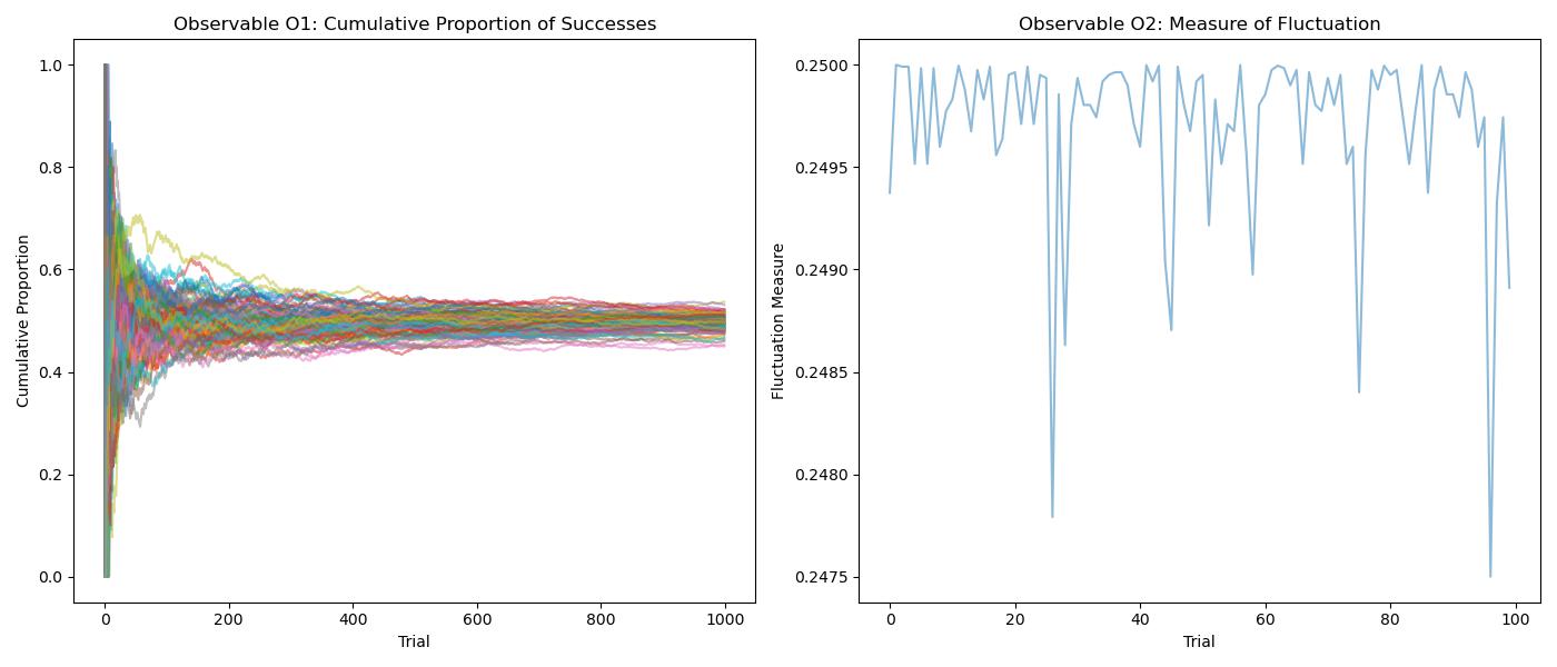
Content Description:

This figure should illustrate the concept of using two different observables, \(O_1\) and \(O_2\), to analyze ergodicity in Bernoulli trials.

The figure could be a schematic or conceptual diagram that shows two panels or sections. One panel represents \(O_1\), the cumulative proportion of successes, and the other represents \(O_2\), a measure of fluctuation or variability in outcomes.

Each panel might include a hypothetical plot showing how each observable evolves over time for a single sequence of Bernoulli trials, highlighting the approach to a steady state or equilibrium that signifies an ergodic regime.

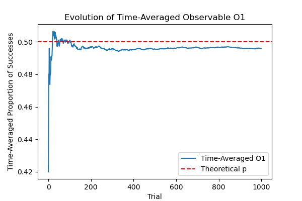
Figure 2: Evolution of Time-Averaged Observable

Content Description:

Figure 2 focuses on the evolution of the time-averaged observable \(O_1\) over a significant number of trials. A graph showing a smooth curve or line that represents the average value of \(O_1\) across multiple sequences of Bernoulli trials as it converges to the theoretical probability of success \(p\). The x-axis represents the number of trials, while the y-axis represents the value of \(O_1\). The plot should ideally show convergence towards \(p\), demonstrating the system’s approach to ergodicity.

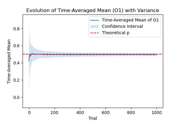
Figure 3: Evolution of Time-Averaged Mean

Content Description:

This figure delves into the specifics of the time-averaged mean of successes, essentially another perspective on \(O_1\), but focusing on its statistical properties over time. A graph depicting the convergence of the time-averaged mean towards the theoretical mean (probability \(p\)) across multiple sequences. This could include error bars or shading to indicate the variance or confidence intervals over time. The visualization should highlight the decrease in variance as the number of trials increases, emphasizing the stabilization of the time-averaged mean in the ergodic regime.

Note: To generate these figures, one would need to execute the provided Python simulation of Bernoulli trials, capturing the evolution of \(O_1\) and \(O_2\) across multiple sequences. The figures are meant to visually convey the theoretical concepts discussed, such as the approach to ergodicity, the role of observables in detecting ergodic regimes, and the significance of time-averaged measures in distinguishing ergodic behavior.

Python Code for Generating the Figures

import numpy as np
import matplotlib.pyplot as plt

# Simulate Bernoulli trials
def simulate_bernoulli_trials(trials, p_success, sequences=1):
    """Simulate sequences of Bernoulli trials."""
    return np.random.binomial(1, p_success, size=(sequences, trials))

# Calculate observables O1 and O2
def calculate_observables(data):
    """Calculate O1 (cumulative proportion of successes) and O2 (fluctuation measure)."""
    O1 = np.cumsum(data, axis=1) / np.arange(1, data.shape[1] + 1)
    O2 = np.var(data, axis=1)  # Simplified measure of fluctuation for demonstration
    return O1, O2

# Plotting functions for the figures
def plot_figures(data, O1, O2, p_success):
    """Plot the figures described in the request."""
    
    # Figure 1: Two Observables' Approach to Ergodicity for Bernoulli Trials
    plt.figure(figsize=(14, 6))
    plt.subplot(1, 2, 1)
    plt.plot(O1.T, alpha=0.5)
    plt.title('Observable O1: Cumulative Proportion of Successes')
    plt.xlabel('Trial')
    plt.ylabel('Cumulative Proportion')
    
    plt.subplot(1, 2, 2)
    plt.plot(O2.T, alpha=0.5)
    plt.title('Observable O2: Measure of Fluctuation')
    plt.xlabel('Trial')
    plt.ylabel('Fluctuation Measure')
    plt.tight_layout()
    plt.show()

    # Figure 2: Evolution of Time-Averaged Observable O1
    plt.figure(figsize=(6, 4))
    plt.plot(O1.mean(axis=0), label='Time-Averaged O1')
    plt.axhline(y=p_success, color='r', linestyle='--', label='Theoretical p')
    plt.title('Evolution of Time-Averaged Observable O1')
    plt.xlabel('Trial')
    plt.ylabel('Time-Averaged Proportion of Successes')
    plt.legend()
    plt.show()

    # Figure 3: Evolution of Time-Averaged Mean with Confidence Intervals
    plt.figure(figsize=(6, 4))
    mean_O1 = O1.mean(axis=0)
    std_O1 = O1.std(axis=0)
    plt.plot(mean_O1, label='Time-Averaged Mean of O1')
    plt.fill_between(range(len(mean_O1)), mean_O1-std_O1, mean_O1+std_O1, alpha=0.2, label='Confidence Interval')
    plt.axhline(y=p_success, color='r', linestyle='--', label='Theoretical p')
    plt.title('Evolution of Time-Averaged Mean (O1) with Variance')
    plt.xlabel('Trial')
    plt.ylabel('Time-Averaged Mean')
    plt.legend()
    plt.show()

# Parameters for simulation
trials = 1000
p_success = 0.5
sequences = 100

# Simulate Bernoulli trials and calculate observables
data = simulate_bernoulli_trials(trials, p_success, sequences)
O1, O2 = calculate_observables(data)

# Plot the figures based on the calculated observables
plot_figures(data, O1, O2, p_success)

Check out Data Science Books on Amazon