Data drift is usually discovered too late. A model begins to make worse predictions, business metrics decline, analysts investigate, and only then does the team realize that the input environment has changed. By that point, the damage has already happened: bad credit decisions, poor demand forecasts, irrelevant recommendations, delayed maintenance alerts, or unnecessary manual reviews.
The difficulty is that the most direct evidence of model degradation often depends on labels, and labels can arrive slowly. Loan default labels may take months. Churn labels may require a full billing cycle. Medical outcomes may take weeks. Even in fast digital systems, high-quality ground truth is often delayed, noisy, or incomplete.
Unsupervised learning is useful because it can monitor the input distribution before labels arrive. It cannot prove that the model is wrong. It can, however, detect that the production data no longer looks like the data used to build, validate, and calibrate the model. That early signal is valuable when it is treated as a trigger for investigation rather than as automatic proof of failure.
What Unsupervised Drift Detection Can and Cannot Do
Unsupervised drift detection answers a specific question:
Does current production data look meaningfully different from the reference data?
It does not directly answer:
Has predictive performance degraded?
The distinction matters. Some shifts are harmless. For example, a retail model may see more weekend traffic during a holiday campaign, but the relationship between customer behavior and purchase probability may remain stable. Other shifts are dangerous. A new acquisition channel may bring users whose behavior is poorly represented in training data, causing calibration errors and biased decisions.
Unsupervised methods should therefore be part of a monitoring hierarchy. They are early warning systems. They help teams decide where to look, which cohorts to inspect, which labels to prioritize, and whether retraining or recalibration should be considered.
Start With the Right Representation
Raw features are not always the best space for drift detection. A production model may have hundreds or thousands of inputs, including sparse categorical variables, text embeddings, behavioral aggregates, and engineered ratios. Monitoring every raw feature separately creates alert noise and misses multivariate changes.
A better approach is to define several monitoring representations:
- Raw critical features for simple sanity checks
- Model input features after preprocessing
- Learned embeddings for text, images, or high-cardinality entities
- Model scores and intermediate representations
- Business cohorts such as channel, geography, customer segment, or device type
Each representation reveals a different kind of shift. Raw features catch instrumentation failures and schema problems. Preprocessed features catch changes seen by the model. Embeddings catch semantic changes that are difficult to monitor feature by feature. Model scores reveal how the model’s risk distribution is moving, even before labels arrive.
The representation should be stable. If preprocessing code changes, drift statistics may change because the measurement process changed, not because production changed. Versioning the feature pipeline is therefore part of drift monitoring.
Clustering as a Drift Sensor
Clustering can detect changes in the composition of production data. The basic idea is simple: learn clusters on reference data, then monitor how new observations distribute across those clusters.
Suppose a model serves five common customer behavior patterns. If production traffic suddenly concentrates in one cluster or begins producing observations far from all known clusters, the system may be seeing a new population.
A practical workflow looks like this:
- Fit a clustering model on reference data.
- Assign each production observation to the nearest cluster.
- Track cluster proportions over time.
- Track distance to assigned cluster centers.
- Alert when proportions or distances move beyond calibrated limits.
Cluster monitoring is useful because it is interpretable. A team can inspect the cluster that changed and ask what is different about it: acquisition source, transaction size, geography, seasonality, product mix, or missing data pattern.
The weakness is that clustering is sensitive to scaling, irrelevant dimensions, and the number of clusters. It should not be treated as a universal detector. It works best when the representation has been engineered for meaningful similarity.
Autoencoders and Reconstruction Error
Autoencoders learn to compress and reconstruct normal reference data. When production observations have high reconstruction error, they may be unlike the reference population.
The useful signal is not the reconstruction error of a single record. Individual anomalies are expected in production. The stronger signal is a sustained change in the distribution of reconstruction errors:
Reference: low and stable reconstruction error
Production: rising median error or heavier upper tail
Autoencoders are attractive for high-dimensional data because they can learn nonlinear structure. They can be effective for sensor streams, embeddings, images, and complex behavioral features.
They also create risks. A powerful autoencoder may reconstruct too many unusual observations well, hiding drift. A weak autoencoder may flag harmless variation. The model may also learn artifacts from the reference period, such as a temporary campaign or an outdated product mix.
For production use, reconstruction error should be monitored by cohort and time window. A global error average can hide localized drift. If only one region, machine type, product category, or user segment is shifting, the overall metric may look stable while the model fails for that subgroup.
Density and Distance Methods
Density estimation and distance-based methods compare the location of current data against the reference distribution. Common approaches include nearest-neighbor distances, kernel density estimates, isolation forests, one-class support vector machines, and embedding-space distance metrics.
These methods are useful when the question is whether current observations occupy familiar regions of feature space. They are particularly helpful when failures are caused by out-of-distribution inputs.
However, high-dimensional distance is difficult. As dimensions increase, distances can become less informative unless the representation is compact and meaningful. That is why embedding design, dimensionality reduction, and feature selection matter more than the choice of detector.
A simple distance method on a good representation often beats a sophisticated detector on a noisy representation.
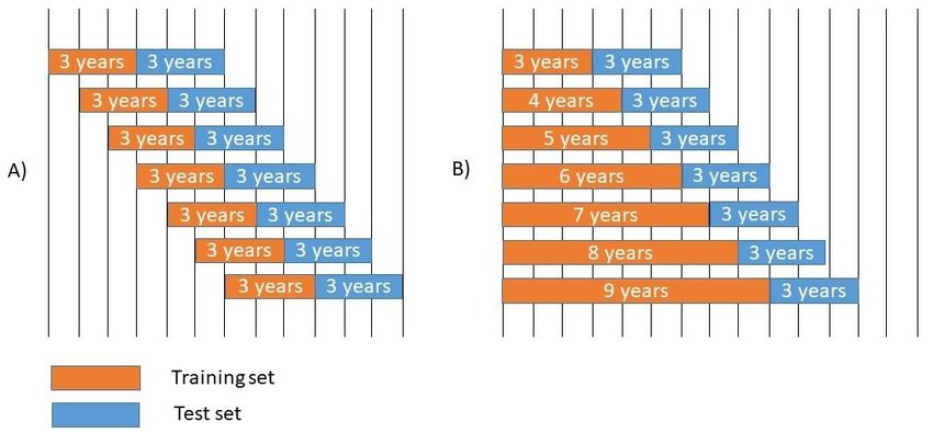
Windowing and Reference Data
Drift detection depends on comparing a current window with a reference window. Choosing those windows is not a trivial detail.
The reference should represent the model’s intended operating environment. It may be the training data, a validation set, a recent stable production period, or a rolling reference. Each choice has trade-offs.
Training data is useful because it reflects what the model learned. But if production has already moved since training, it may create constant alerts. A recent stable production window may be operationally realistic, but it can normalize gradual drift and forget the original modeling assumptions.
Window size also matters. Short windows detect changes quickly but create more false alarms. Long windows are stable but slow. A mature monitoring system often uses multiple windows:
- Short window for abrupt shifts
- Medium window for emerging trends
- Long window for slow structural movement
The system should also respect seasonality. Comparing Monday morning traffic with weekend traffic may create artificial drift alerts. When seasonality is strong, compare like with like.
Calibrating Alerts
The most damaging failure mode in drift monitoring is alert fatigue. If the system alerts constantly, teams stop responding. An unsupervised detector must therefore be calibrated around operational capacity.
Good alert design includes:
- Severity levels rather than one binary alarm
- Cohort attribution showing where the shift occurred
- Evidence explaining which features or representations changed
- Suppression rules for known events
- Escalation only after persistence across windows
- Feedback from investigations
An alert should not merely say that a metric crossed a threshold. It should tell the team what changed, when it changed, which population changed, and how large the affected volume is.
Thresholds should be set using historical backtesting. Run the detector over past stable periods and known change periods. Estimate how often it would have alerted, how early it would have detected known incidents, and how many alerts the team would have had to investigate.
Connecting Drift to Action
Detection is not the end of the workflow. A drift signal should trigger a decision tree:
- Is the shift caused by a data quality issue?
- Is the shift expected because of seasonality, campaign activity, or product change?
- Is the affected cohort important enough to investigate immediately?
- Do early outcome proxies suggest performance risk?
- Should labels be sampled or reviewed faster for the affected cohort?
- Is recalibration, retraining, or feature repair needed?
This action layer is where many monitoring programs fail. They build dashboards but do not define ownership. A useful drift system names who investigates, what evidence they inspect, and when the issue escalates.
Combining Unsupervised and Supervised Signals
Unsupervised methods should eventually be reconciled with labels. When labels arrive, the team should ask whether earlier drift signals predicted actual degradation. This creates a learning loop:
- Drift alert occurred
- Investigation found affected cohort
- Labels later confirmed or rejected performance degradation
- Detector threshold or representation was adjusted
Over time, this feedback helps distinguish harmless distribution movement from shifts that matter for model quality. The goal is not to eliminate all false positives. The goal is to make alerts increasingly relevant to real operational risk.
Conclusion
Unsupervised learning can make data drift visible before labels arrive, but it must be used with discipline. Clustering, reconstruction error, density methods, and embedding distances are not magic detectors. They are measurement tools whose value depends on representation quality, window design, threshold calibration, cohort analysis, and response workflow.
The best systems treat unsupervised drift detection as an early warning layer. They do not ask it to prove model failure. They ask it to reveal when production data has moved far enough from familiar territory that the organization should look closer, collect evidence faster, and decide whether the model still deserves trust.