Time series data often combine several underlying components: a long-term trend, repeating seasonal patterns, and random residual noise. By decomposing a series into these pieces, you can better understand its behavior and build more accurate forecasts.
Additive vs. Multiplicative Models
In an additive model, the components simply add together:
\[y_t = T_t + S_t + R_t\]where $T_t$ is the trend, $S_t$ is the seasonal component, and $R_t$ represents the residuals. A multiplicative model instead multiplies these terms:
\[y_t = T_t \times S_t \times R_t\]Choose the form that best fits the scale of seasonal fluctuations in your data.
The diagnostic is straightforward: plot the series and look at the seasonal swings over time. If the peaks and troughs keep a roughly constant absolute size as the level rises, the structure is additive. If they grow proportionally with the level, so that a busy December is always about 40% above trend rather than always 5,000 units above it, the structure is multiplicative.
The two are related by a logarithm. Taking logs of a multiplicative series gives
\[\log y_t = \log T_t + \log S_t + \log R_t,\]which is additive. Modelling the log of a series and then back-transforming is often simpler than handling multiplicative components directly, though remember that exponentiating a forecast of the mean log does not give the mean of the original scale.
Classical Decomposition and Its Limits
The traditional algorithm is easy to follow. Estimate the trend with a centred moving average whose window equals the seasonal period. Remove it from the series. Average the detrended values by seasonal position to get the seasonal indices. Whatever remains is the residual.
Two weaknesses follow directly from that construction. A centred moving average of period $m$ cannot produce values for the first and last $m/2$ observations, so the trend is undefined at both ends of the series, exactly where forecasting cares most. And averaging by seasonal position forces the seasonal pattern to be identical in every cycle, which fails whenever seasonality genuinely evolves, as retail and energy demand usually do.
Extracting the Components
Python libraries like statsmodels or pandas offer built-in functions to perform decomposition. Once the trend and seasonality are isolated, you can analyze them separately or remove them before applying forecasting models such as ARIMA.
import pandas as pd
from statsmodels.tsa.seasonal import seasonal_decompose, STL

series = pd.read_csv("sales.csv", index_col="date", parse_dates=True)["units"]
series = series.asfreq("MS")            # explicit frequency is required

classical = seasonal_decompose(series, model="multiplicative", period=12)
classical.plot()

stl = STL(series, period=12, robust=True).fit()
components = pd.DataFrame({
    "trend": stl.trend,
    "seasonal": stl.seasonal,
    "residual": stl.resid,
})
STL, which stands for Seasonal-Trend decomposition using Loess, addresses both weaknesses of the classical approach. It estimates components with local regression rather than fixed moving averages, so it produces values across the full span of the series. It allows the seasonal component to change gradually, controlled by the seasonal smoothing parameter. And with robust=True it downweights outliers, preventing a single anomalous month from bending the trend or contaminating every future estimate of that season.
STL is additive by construction, so apply it to log-transformed data when the pattern is multiplicative.
Reading the Residuals
The residual component is the most useful diagnostic in the output, because it is what the decomposition failed to explain. Well-behaved residuals look like noise: no visible trend, no repeating cycle, roughly constant variance.
Structure that survives into the residuals tells you something specific. A remaining cycle usually means the period was set wrong, or that a second seasonality exists, such as weekly and annual patterns in daily data. Variance that grows with the level means an additive model was applied to a multiplicative series. Isolated spikes mark genuine events such as promotions, outages, or holidays, and those are often worth modelling explicitly as regressors rather than leaving as unexplained noise.
Formally, an Ljung-Box test on the residuals checks whether any autocorrelation remains, and a significant result means predictable structure has been left on the table.
Where Decomposition Fits in Forecasting
Decomposition serves three distinct purposes, and it is worth being clear about which one you are using.
As explanation, it separates a headline number into parts a stakeholder can reason about. “Sales rose 8%” becomes “underlying demand rose 3% while the seasonal peak accounted for the rest”, which is a far more actionable statement.
As preprocessing, it produces a seasonally adjusted series. Removing seasonality before fitting a model lets that model concentrate on the trend and any remaining dynamics, which is exactly what official statistics agencies do when they publish adjusted unemployment or retail figures.
As forecasting, the components can be projected separately and recombined: extrapolate the trend, repeat the seasonal pattern, and assume the residual has mean zero. This works, but it treats the decomposition as exact and ignores uncertainty in the component estimates, so prediction intervals from this route are usually too narrow. Methods that estimate components and forecasts jointly, such as exponential smoothing state space models or SARIMA, handle that coherently and are the better choice when interval accuracy matters.
Practical Cautions
Set the period from domain knowledge rather than letting a default decide. Monthly data with annual seasonality has period 12; daily data may need 7 for weekly effects, 365.25 for annual effects, or both via MSTL. Series with multiple seasonalities cannot be handled by a single-period decomposition at all.
Decomposition is descriptive, not causal. A rising trend component describes what happened; it does not explain why, and extrapolating it assumes the underlying cause persists.
Finally, be careful when decomposing a series you intend to evaluate a forecast against. Fitting the decomposition on the full series, including the test period, leaks future information into the components and will make backtest results look better than they are.
Understanding each component allows you to explain past observations and produce more transparent predictions for future values.
References
- Hyndman, R. J., & Athanasopoulos, G. (2021). Forecasting: Principles and Practice (3rd ed.). OTexts.
- Cleveland, R. B., Cleveland, W. S., McRae, J. E., & Terpenning, I. (1990). STL: A seasonal-trend decomposition procedure based on loess. Journal of Official Statistics, 6(1), 3-73.
- Bandara, K., Hyndman, R. J., & Bergmeir, C. (2021). MSTL: A seasonal-trend decomposition algorithm for time series with multiple seasonal patterns. arXiv:2107.13462.
- Ljung, G. M., & Box, G. E. P. (1978). On a measure of lack of fit in time series models. Biometrika, 65(2), 297-303.