At the end of this blog, you will be able to visually explain the variance in your data, select the most informative features, and create insightful plots. We will cover the following topics in detail:
-
Feature Selection vs. Extraction
Understand the fundamental differences between feature selection and feature extraction, and learn when to apply each technique for optimal results. -
Dimension Reduction Using PCA
Explore how Principal Component Analysis (PCA) effectively reduces dimensionality in datasets while preserving essential information. -
Explained Variance and the Scree Plot
Learn to calculate and interpret the explained variance to understand how much information each principal component captures. Use scree plots to visualize this distribution. -
Loadings and the Biplot
Discover how loadings represent the contribution of each original feature to the principal components and how biplots can visualize these relationships. -
Extracting the Most Informative Features
Identify and extract the features that contribute the most to your data’s variability and use this information to enhance model performance and interpretability. -
Outlier Detection
Utilize PCA to detect outliers in your data, improving the overall quality and robustness of your analysis.
By the end of this guide, you will have a thorough understanding of PCA and its applications, enabling you to make more informed decisions in your data analysis and machine learning projects.
Gentle Introduction to PCA
The main purpose of Principal Component Analysis (PCA) is to reduce dimensionality in datasets while minimizing information loss. High-dimensional data can be challenging to analyze due to the curse of dimensionality, where the performance of classifiers and other models deteriorates as the number of features increases. PCA addresses this issue by transforming the data into a new set of dimensions, known as principal components, which are linear combinations of the original features.
There are two primary methods to reduce dimensionality: Feature Selection and Feature Extraction. Understanding the distinction between these methods is crucial:
-
Feature Selection: This method involves selecting a subset of the original features that are most informative for the task at hand. This subset should contain the most relevant information while discarding redundant or irrelevant features. Feature selection is beneficial when the goal is to maintain the interpretability of the original features and is often used in scenarios where the features have different units or scales.
-
Feature Extraction: Unlike feature selection, feature extraction creates new features by combining the original features. PCA is a prime example of this method. It constructs new dimensions (principal components) that capture the maximum variance in the data. These new dimensions are uncorrelated and ordered by the amount of variance they explain, with the first principal component explaining the most variance.
Reducing dimensionality is important for several reasons:
- Reducing Complexity: Simplifies the model, making it easier to interpret and faster to train.
- Improving Run Time: Decreases the computational load, leading to quicker analyses.
- Determining Feature Importance: Helps identify which features contribute the most to the outcome.
- Visualizing Class Information: Facilitates the visualization of high-dimensional data in 2D or 3D plots.
- Preventing the Curse of Dimensionality: Improves model performance by avoiding overfitting and enhancing generalization.
Choosing between feature selection and feature extraction depends on the specific needs of your analysis. Feature selection is preferable when maintaining the original features’ interpretability is important. In contrast, feature extraction, such as PCA, is useful when the goal is to capture the maximum variance with fewer dimensions, even if it means losing some interpretability.
In the next section, we will delve deeper into how to choose between feature selection and feature extraction techniques, providing insights into their respective advantages and applications.
Feature Selection
Feature selection is a crucial process in data preprocessing that involves identifying and selecting a subset of the most relevant features from the original dataset. This process is necessary in several situations:
- Non-Numeric Features: When the dataset includes non-numeric features, such as strings or categorical data, feature selection helps in identifying the most relevant features that can be converted into numeric representations for analysis.
- Meaningful Features: When the goal is to retain the most meaningful features that contribute significantly to the target variable or the outcome of interest. This is particularly important in domains where interpretability is critical, such as healthcare or finance.
- Measurement Integrity: When it is essential to keep the original measurements intact. A transformation, such as that used in feature extraction, would result in a linear combination of measurements, leading to the loss of the original units and making it difficult to interpret the results.
While feature selection is highly beneficial, it has some disadvantages. One major drawback is that it requires a search strategy and/or an objective function to evaluate and select potential candidates. This often involves computational complexity and can be time-consuming. For instance, it may require a supervised approach with class information to perform a statistical test or a cross-validation approach to identify the most informative features.
However, feature selection can also be performed without class information. In such cases, unsupervised methods can be used, such as selecting the top N features based on variance, where higher variance is often an indicator of greater informational value. This approach is simpler but may not always capture the most relevant features for the specific task.
Common Feature Selection Methods
-
Filter Methods: These methods apply a statistical measure to assign a scoring to each feature. Features are ranked by the score, and either selected to be kept or removed from the dataset. Examples include correlation coefficients, chi-square tests, and mutual information.
-
Wrapper Methods: These methods evaluate the feature subsets using a machine learning model. They are computationally intensive but often provide better performance. Examples include recursive feature elimination and forward/backward feature selection.
-
Embedded Methods: These methods perform feature selection during the model training process. Examples include regularization methods like Lasso (L1) and Ridge (L2) regression, which penalize certain features during model fitting.
Feature selection is a powerful tool to enhance model performance, improve interpretability, and reduce overfitting by eliminating irrelevant or redundant features. Choosing the right method and approach depends on the specific characteristics of the dataset and the goals of the analysis.
Feature Extraction
Feature extraction is a dimensionality reduction technique that transforms the original features into a new set of features while minimizing the loss of information. This approach is particularly useful when dealing with high-dimensional data, as it reduces the number of dimensions and helps to avoid the curse of dimensionality. In the context of Principal Component Analysis (PCA), feature extraction is achieved through a linear transformation.
The transformation function in PCA can be expressed as \(y = f(x)\), which is rewritten as \(y = Wx\). Here, \(W\) represents the weights or coefficients of the linear combination, \(x\) are the input features, and \(y\) is the final transformed feature space. The primary goal of this transformation is to capture the maximum variance in the data with the fewest principal components.
Steps in PCA for Feature Extraction
-
Standardization: Before applying PCA, it is essential to standardize the data to ensure that each feature contributes equally to the analysis. This involves rescaling the features to have a mean of zero and a standard deviation of one.
-
Covariance Matrix Computation: Calculate the covariance matrix to understand how the variables in the dataset vary with respect to each other.
-
Eigenvalue and Eigenvector Calculation: Compute the eigenvalues and eigenvectors of the covariance matrix. The eigenvectors determine the directions of the new feature space, while the eigenvalues indicate the magnitude of the variance in these directions.
-
Forming Principal Components: Sort the eigenvalues in descending order and select the top k eigenvectors to form the principal components. These principal components are the new features that capture the most significant variance in the data.
-
Transforming the Data: Finally, transform the original data into the new feature space defined by the principal components.
Advantages of Feature Extraction
- Dimensionality Reduction: Significantly reduces the number of features while retaining most of the original data’s variability.
- Improved Model Performance: Reduces overfitting and improves the performance of machine learning models by eliminating noise and redundant information.
- Enhanced Visualization: Facilitates the visualization of high-dimensional data in 2D or 3D plots.
Disadvantages of Feature Extraction
Despite its advantages, feature extraction, particularly through PCA, has some drawbacks:
-
Loss of Interpretability: The transformed features (principal components) are linear combinations of the original features, making them less interpretable. For instance, if potential cancer-related genes are discovered using PCA, it may be challenging to pinpoint the exact contribution of each gene.
-
Follow-up Challenges: In certain use cases, such as biomedical research, the lack of interpretability can hinder follow-up actions. For example, if a combination of genes is identified as significant, it may not be feasible to target individual genes for experimental validation.
Feature extraction through PCA is a powerful technique for reducing dimensionality and enhancing the performance of data analysis. However, it is essential to consider the trade-off between reducing dimensions and maintaining interpretability, especially in applications where understanding the contribution of individual features is crucial.
How Are Dimensions Reduced in PCA?
Principal Component Analysis (PCA) is a technique used to reduce the dimensionality of datasets by transforming the original features into a new set of features called principal components. These components are orthogonal and capture the maximum variance in the data. The process of dimension reduction in PCA can be broken down into several key steps:
Part 1: Center Data Around the Origin
The first step in PCA is to center the data around the origin. This involves computing the mean of the data and then subtracting this mean from each data point. The steps are as follows:
- Compute the average per feature: Calculate the mean value for each feature in the dataset.
- Compute the overall center: Determine the center of the dataset by averaging the means of all features.
- Shift the data: Subtract the mean value of each feature from the corresponding feature values in the dataset.
This transformation centers the data around the origin (mean of zero) without altering the relative distances between the data points.
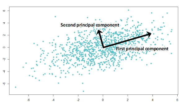
Part 2: Fit the Line Through Origin and Data Points
Next, we fit a line through the origin and the data points. This line represents the direction of maximum variance in the data. The steps are:
- Draw a random line through the origin: Start with a line passing through the origin.
- Project the samples on the line orthogonally: Project each data point onto the line at right angles.
- Rotate until the best fit is found: Adjust the orientation of the line to minimize the sum of squared distances (SS) from the data points to the line. This maximizes the variance along the line.
Part 3: Computing the Principal Components and the Loadings
Once the line representing the direction of maximum variance (the first principal component, PC1) is found, we compute the slope of PC1, which describes the contribution of each feature to PC1. The steps include:
- Compute the eigenvectors and eigenvalues: Calculate the eigenvectors and eigenvalues of the covariance matrix of the centered data. The eigenvectors represent the directions of maximum variance, while the eigenvalues represent the magnitude of variance in these directions.
- Form the principal components: The eigenvector with the highest eigenvalue becomes the first principal component (PC1). The next eigenvector with the highest eigenvalue becomes the second principal component (PC2), and so on.
The loadings are the coefficients of the linear combination of the original features that make up each principal component. They indicate the contribution of each feature to the principal component.
Part 4: The Transformation and Explained Variance
After computing the principal components, the entire dataset is transformed into the new feature space defined by these components. The steps are:
- Transform the dataset: Multiply the original data matrix by the matrix of eigenvectors to obtain the principal component scores.
- Compute the explained variance: For each principal component, calculate the proportion of the total variance it explains. This is done by dividing the sum of squared distances (SS) for each principal component by the number of data points minus one.
The explained variance helps in understanding how much information (variance) each principal component captures from the original data.
Standardization
Before performing PCA, it is crucial to standardize the data. Standardization ensures that each feature contributes equally to the analysis by rescaling the features to have a mean of zero and a standard deviation of one. This step is necessary because PCA is sensitive to variables with different scales or the presence of outliers. Standardization can be achieved by:
- Subtracting the mean: Subtract the mean value of each feature from the corresponding feature values.
- Dividing by the standard deviation: Divide each feature value by the standard deviation of the feature.
By standardizing the data, we ensure that each feature has the properties of a standard normal distribution, allowing PCA to accurately capture the underlying structure of the data.
Understanding these steps provides a comprehensive view of how PCA reduces dimensionality and transforms the data into a new feature space that retains the most significant information.
The PCA Library
The pca library is a versatile tool designed to simplify and enhance the process of Principal Component Analysis. It provides a comprehensive set of functionalities to address various challenges encountered during PCA analysis. The key features of the pca library include:
- Analyzing Different Types of Data: The library supports a wide range of data types, making it suitable for diverse datasets.
- Computing and Plotting Explained Variance: It allows users to compute the explained variance and visualize it using scree plots, facilitating the interpretation of how much variance each principal component captures.
- Extraction of Best-Performing Features: The library helps identify and extract the most informative features, improving model performance and interpretability.
- Insights into Loadings with the Biplot: Users can gain insights into the contributions of original features to the principal components through biplots.
- Outlier Detection: The library includes methods for detecting outliers, enhancing the robustness of the analysis.
- Removal of Unwanted (Technical) Bias: It provides functionalities to normalize data and remove technical biases, ensuring a more accurate analysis.
Benefits of pca Library
The pca library offers several benefits that make it a preferred choice for PCA analysis:
- Maximizes Compatibility and Integration in Pipelines: Built on top of the widely-used
scikit-learnlibrary,pcaensures seamless integration into existing data science workflows and pipelines. - Built-in Standardization: The library includes built-in standardization, simplifying the preprocessing steps required before performing PCA.
- Comprehensive Output and Plots: It generates the most sought-after outputs and plots, including scree plots, biplots, and explained variance plots, making it easier to interpret and present the results.
- Simple and Intuitive: The library is designed to be user-friendly, with an intuitive API that simplifies the PCA process even for those new to the technique.
- Open-Source with Comprehensive Documentation: As an open-source library,
pcais freely available and comes with extensive documentation, including numerous examples, ensuring that users can easily learn and apply PCA to their datasets.
The pca library streamlines the process of performing PCA, offering powerful tools and visualizations to enhance the understanding and interpretation of high-dimensional data. Whether you are looking to reduce dimensionality, identify key features, or detect outliers, the pca library provides the necessary functionalities to achieve these goals efficiently.
A Practical Example to Understand the Loadings
Creating a Synthetic Dataset
To understand the principles of PCA, we will start by creating a synthetic dataset. This dataset will contain 8 features and 250 samples. Each feature will consist of random integers with increasing variance, ensuring all features are independent of each other. This synthetic dataset is ideal for demonstrating PCA principles, including the loadings, the explained variance, and the importance of standardization.
Here is the code to generate the synthetic dataset:
import numpy as np
import pandas as pd

# Setting the seed for reproducibility
np.random.seed(42)

# Creating a synthetic dataset with 8 features and 250 samples
data = {
    'feature1': np.random.randint(0, 100, 250),
    'feature2': np.random.randint(0, 50, 250),
    'feature3': np.random.randint(0, 25, 250),
    'feature4': np.random.randint(0, 12, 250),
    'feature5': np.random.randint(0, 6, 250),
    'feature6': np.random.randint(0, 3, 250),
    'feature7': np.random.randint(0, 2, 250),
    'feature8': np.random.randint(0, 1, 250)
}

# Creating a DataFrame
df = pd.DataFrame(data)
PCA Results
After generating the dataset, the next step is to fit and transform the data using PCA. This process will help us examine the features and their variation. We will visualize the explained (cumulative) variance with a scree plot and create a 2-dimensional plot to visualize the loadings and scatter.
Here is the code to perform PCA and visualize the results:
from pca import pca
import matplotlib.pyplot as plt

# Initialize PCA model
model = pca(n_components=None)

# Fit and transform the data
results = model.fit_transform(df)

# Plot explained variance
model.plot()
plt.show()

# Plot the PCA biplot
model.biplot()
plt.show()
Real Dataset: Wine Dataset
To further illustrate PCA, we will analyze the wine dataset, which is more realistic. The wine dataset contains 178 samples, 13 features, and 3 wine classes. Normalizing the data ensures that each variable contributes equally to the analysis. By applying PCA to this dataset, we can extract the top-performing features and visualize the explained variance with a scree plot.
Here is the code to analyze the wine dataset:
from sklearn.datasets import load_wine

# Load the wine dataset
wine = load_wine()
wine_df = pd.DataFrame(wine.data, columns=wine.feature_names)

# Initialize PCA model with normalization
model = pca(n_components=None, normalize=True)

# Fit and transform the wine data
results = model.fit_transform(wine_df)

# Plot explained variance for the wine dataset
model.plot()
plt.show()

# Plot the PCA biplot for the wine dataset
model.biplot(label=wine.target)
plt.show()
In the wine dataset analysis, the scree plot will show how the variance is distributed among the principal components. The biplot will help us understand the contributions of each original feature to the principal components, revealing insights into the data’s underlying structure.
By following these steps, you can gain a practical understanding of how PCA works, how to interpret the loadings, and how to visualize the explained variance and contributions of features in both synthetic and real datasets.
Outlier Detection
Outlier detection is an essential aspect of data analysis, as outliers can significantly impact the results and interpretations of your models. The pca library provides two robust methods for detecting outliers: Hotelling’s T2 and SPE/DmodX. These methods complement each other, and by computing the overlap between them, you can identify the most deviant observations with greater accuracy.
Hotelling’s T2 Method
Hotelling’s T2 method is a multivariate statistical approach used to identify outliers based on the Mahalanobis distance. This method evaluates the distance of each data point from the center of the dataset, taking into account the covariance structure of the data. Points that are far from the center, as measured by this multivariate distance, are considered outliers.
How It Works
-
Calculate the Mean Vector and Covariance Matrix: The mean vector and covariance matrix of the dataset are computed. The mean vector represents the center of the dataset, and the covariance matrix captures the relationships between the variables.
-
Compute Mahalanobis Distance: For each data point, the Mahalanobis distance is calculated. This distance measures how many standard deviations away a point is from the mean of the dataset, considering the covariance structure. The formula for the Mahalanobis distance \(D^2\) for a data point \(x\) is given by: \(D^2 = (x - \mu)^T \Sigma^{-1} (x - \mu)\) where \(\mu\) is the mean vector and \(\Sigma\) is the covariance matrix.
-
Determine Threshold: A threshold is set to distinguish between normal observations and outliers. This threshold is typically based on the chi-squared distribution with degrees of freedom equal to the number of variables. Observations with a Mahalanobis distance exceeding this threshold are considered outliers.
-
Identify Outliers: Data points with Mahalanobis distances above the threshold are flagged as outliers. These points lie far from the center of the data distribution.
Benefits
- Considers Multivariate Structure: Hotelling’s T2 method accounts for the covariance structure of the data, making it more robust in identifying outliers in multivariate settings compared to univariate methods.
- Statistical Foundation: The method is based on statistical principles, providing a theoretically sound approach to outlier detection.
- Sensitivity to Multivariate Distance: By focusing on the multivariate distance from the center of the data, Hotelling’s T2 can detect outliers that may not be identified by univariate methods.
- Threshold-Based Detection: The use of a threshold allows for a clear distinction between normal observations and outliers, simplifying the identification process.
SPE/DmodX Method
The SPE (Squared Prediction Error) or DmodX method identifies outliers by measuring the deviation of each observation from the PCA model. This method calculates the error between the actual data points and the values predicted by the PCA model. Large errors indicate that the points do not fit well within the principal component space, marking them as outliers.
How It Works
-
PCA Model Construction: First, a PCA model is built using the training data. The principal components are derived from this model, capturing the directions of maximum variance in the dataset.
-
Prediction and Error Calculation: For each observation, the PCA model predicts the values based on the principal components. The squared prediction error (SPE) is calculated as the squared difference between the actual data points and the predicted values.
-
Threshold Determination: A threshold is set to distinguish between normal observations and outliers. Observations with an SPE exceeding this threshold are considered outliers. This threshold can be determined statistically or based on domain knowledge.
-
Outlier Identification: Observations with SPE values above the threshold are flagged as outliers. These points deviate significantly from the PCA model, indicating they do not conform to the general data structure.
Benefits
- Sensitivity to Model Fit: The SPE/DmodX method is sensitive to how well the data fits within the principal component space. It identifies points that deviate from the expected pattern, making it effective for detecting anomalies.
- Complementary to Hotelling’s T2: When used alongside Hotelling’s T2 method, SPE/DmodX provides a comprehensive outlier detection approach. Hotelling’s T2 focuses on multivariate distance, while SPE/DmodX highlights deviations from the model fit.
Complementary Use of Both Methods
Using both Hotelling’s T2 and SPE/DmodX methods provides a more comprehensive approach to outlier detection. While Hotelling’s T2 focuses on the overall distance in the multivariate space, SPE/DmodX highlights deviations from the PCA model. Observations identified as outliers by both methods are likely to be the most deviant and warrant further investigation.
Wrapping Up
Principal Component Analysis (PCA) is a powerful technique for reducing dimensionality in datasets, capturing the essential variance in the data while minimizing information loss. Each Principal Component (PC) is a linear combination of the original features, with the coefficients (loadings) indicating the contribution of each feature to the component.
Understanding the loadings is crucial for interpreting the principal components. The loadings can be visualized using biplots, which show the relationships between the original features and the principal components. Biplots help in identifying which features contribute the most to the variation captured by each principal component, providing valuable insights into the structure of the data and the separability of different classes.
The pca library facilitates these analyses by offering robust tools for:
- Computing and Visualizing Principal Components: The library enables the calculation of principal components and their associated loadings, allowing for a detailed examination of how the original features contribute to the components.
- Explained Variance: It helps in understanding how much of the total variance in the data is captured by each principal component, often visualized through scree plots.
- Biplots: These plots provide a visual representation of the loadings and the scores of the principal components, aiding in the interpretation of the PCA results.
- Outlier Detection: Using methods like Hotelling’s T2 and SPE/DmodX, the library helps identify outliers that could skew the analysis, ensuring the robustness of the results.
- Normalization: The built-in standardization functionality ensures that all features contribute equally to the PCA, removing unwanted technical variance or bias.
By integrating these functionalities, the pca library offers a comprehensive toolkit for performing PCA, making it accessible and intuitive even for those new to the technique. Whether you aim to reduce dimensionality, identify key features, or detect outliers, the pca library provides the necessary tools to enhance your data analysis.
In summary, PCA transforms high-dimensional data into a lower-dimensional space while preserving the most significant variance. The loadings and biplots facilitate the interpretation of the principal components, providing clear insights into the data’s structure. The pca library streamlines these processes, offering a powerful and user-friendly solution for PCA analysis.
By mastering PCA and utilizing the pca library, you can effectively reduce dimensionality, improve model performance, and gain deeper insights into your data, ultimately leading to more informed and accurate analyses.
Appendix: Python Code
Hotelling’s T2 Method
import pandas as pd
from pca import pca
from sklearn.datasets import load_wine

# Load the wine dataset
wine = load_wine()
wine_df = pd.DataFrame(wine.data, columns=wine.feature_names)

# Initialize PCA model with normalization
model = pca(n_components=None, normalize=True)

# Fit and transform the wine data
results = model.fit_transform(wine_df)

# Detect outliers using the Hotelling’s T2 method
outliers_t2 = model.compute_outliers(method='t2')

# Plot outliers
model.biplot(label=wine.target, legend=False, cmap='seismic')
plt.scatter(wine_df.iloc[outliers_t2.index].iloc[:, 0],
            wine_df.iloc[outliers_t2.index].iloc[:, 1],
            color='blue', label='Hotelling’s T2 Outliers')
plt.legend()
plt.show()

print("Outliers identified by the Hotelling’s T2 method:", outliers_t2.index)
SPE/DmodX Method
import pandas as pd
from pca import pca
from sklearn.datasets import load_wine

# Load the wine dataset
wine = load_wine()
wine_df = pd.DataFrame(wine.data, columns=wine.feature_names)

# Initialize PCA model with normalization
model = pca(n_components=None, normalize=True)

# Fit and transform the wine data
results = model.fit_transform(wine_df)

# Detect outliers using the SPE/DmodX method
outliers_spe = model.compute_outliers(method='spe')

# Plot outliers
model.biplot(label=wine.target, legend=False, cmap='seismic')
plt.scatter(wine_df.iloc[outliers_spe.index].iloc[:, 0],
            wine_df.iloc[outliers_spe.index].iloc[:, 1],
            color='red', label='SPE Outliers')
plt.legend()
plt.show()

print("Outliers identified by the SPE/DmodX method:", outliers_spe.index)


